The goal is to study whether there is an association between the body size and the number of reproductive success, i.e., does lifetime reproductive success increase with ewe body mass?
8.0.1 Data wrangling and exploration
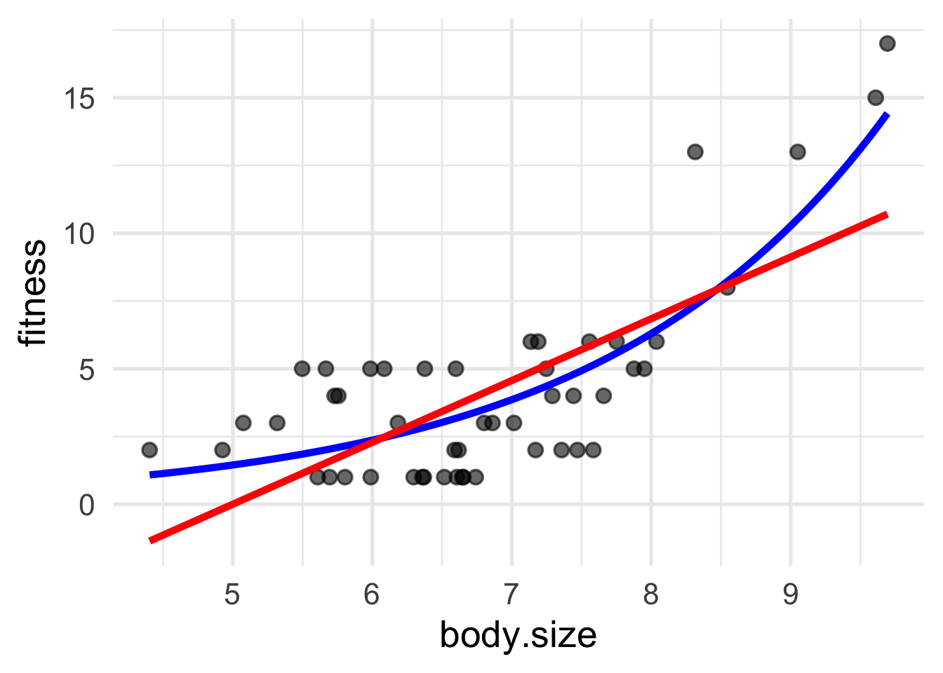
We can visualize the relationship between lifetime reproductive sucess and body mass
Fit a simple linear model. What does the plot Residuals vs Fitted tell you?
Solution
fit1 <-lm(fitness ~ body.size, data = soay)summary(fit1)
Call:
lm(formula = fitness ~ body.size, data = soay)

Residuals:
    Min      1Q  Median      3Q     Max
-3.8965 -1.9029 -0.7107  2.2464  6.2924

Coefficients:
            Estimate Std. Error t value Pr(>|t|)
(Intercept) -11.4021     2.2564  -5.053 6.73e-06 ***
body.size     2.2808     0.3268   6.979 7.91e-09 ***
---
Signif. codes:  0 '***' 0.001 '**' 0.01 '*' 0.05 '.' 0.1 ' ' 1

Residual standard error: 2.577 on 48 degrees of freedom
Multiple R-squared:  0.5037,    Adjusted R-squared:  0.4933
F-statistic: 48.71 on 1 and 48 DF,  p-value: 7.906e-09
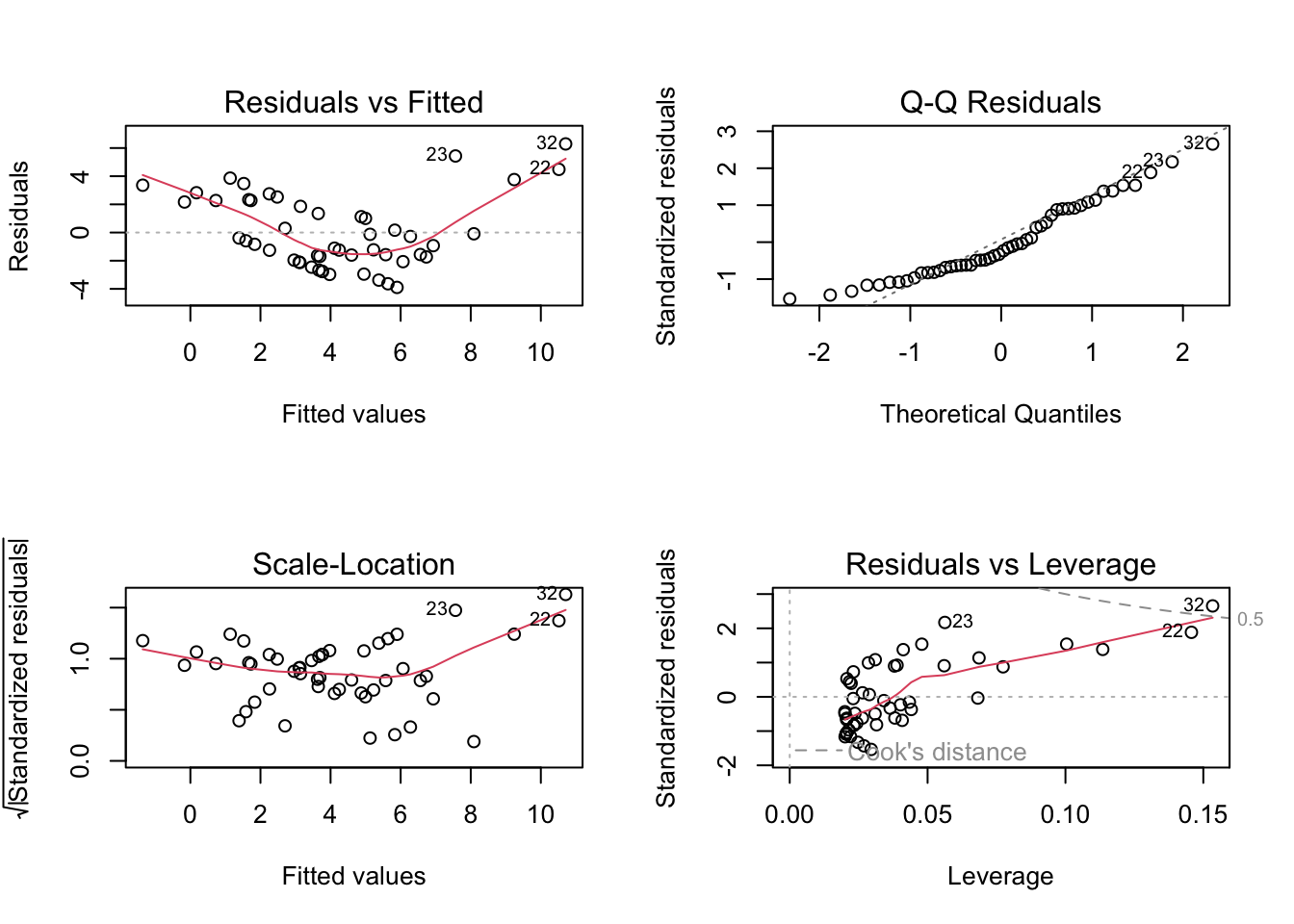
par(mfrow=c(2,2))plot(fit1)
From the Residuals vs Fitted plot, we can see there exist a nonlinearity relationship between fitness and body.size. Therefore, a different approach may be necessary.
8.0.2 Fit a Poisson regression model
fit2 <-glm(fitness ~ body.size, family ="poisson", data = soay)summary(fit2)
Call:
glm(formula = fitness ~ body.size, family = "poisson", data = soay)

Coefficients:
            Estimate Std. Error z value Pr(>|z|)
(Intercept)  -2.0770     0.4256  -4.880 1.06e-06 ***
body.size     0.4896     0.0560   8.743  < 2e-16 ***
---
Signif. codes:  0 '***' 0.001 '**' 0.01 '*' 0.05 '.' 0.1 ' ' 1

(Dispersion parameter for poisson family taken to be 1)

    Null deviance: 125.589  on 49  degrees of freedom
Residual deviance:  53.653  on 48  degrees of freedom
AIC: 208.46

Number of Fisher Scoring iterations: 5
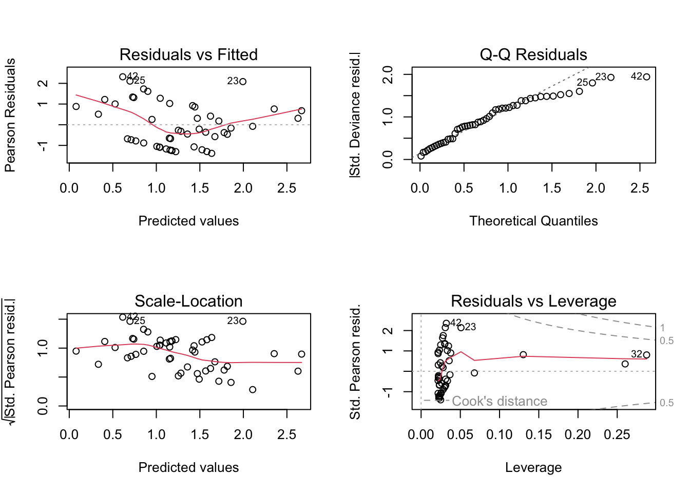
par(mfrow=c(2,2))plot(fit2)
Exercise
What does the output of Poisson regression tell you?
The fitted model is \[\log(\lambda)=-2.0770 + 0.4896 \text{ body.size}\] These results suggest that by exponentiating the coefficient on body.size, we obtain the multiplicative factor by which the mean count changes. In this case, the mean number of offspring born changes by a factor of \(\exp(0.4896)=1.631663\) or increases 63.17% (since $1.631663-1=0.63166) if a body mass increase 1.
The total deviance for NULL (fitness), and the deviance reduce \(125.589−53.653=71.936\) if we consider the body size as a predictor. This is a large reduction, meaning the predictor explains a lot of variation, i.e., the body size is an important predictor of fitness. We can verify this conclusion by perform a deviance test.
The test statistic has a value of 71.936, corresponding p value is very small. This means that adding predictor (body.size) significantly improves the model.
8.0.3 Prediction
Let’s go back to parameter estimation. Here, we have estimated the two regression coefficients, we can also compute confidence intervals for those estimates.
This allows us to be more confident on the inferential statements about the relation between the lifetime reproductive success and the body size.
However, very often one of the goals of generalized linear model is prediction. For instance, we can try and predict what would be the number of number of offspring produced by an ewe that has body size is 6, 7, 8 in average.
# for body.size = 6exp(-2.0770+0.4896*6)
[1] 2.364579
# for body.size = 6exp(-2.0770+0.4896*7)
[1] 3.858197
# for body.size = 6exp(-2.0770+0.4896*8)
[1] 6.295279
Exercise
Predict the number of number of offspring produced by a ewe that has body size is 6, 7, 8 using predict() function. What do you notice?
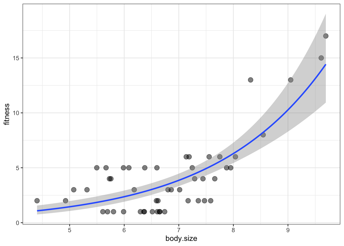
8.0.4 Plotting the fitted curve
min.size <-min(soay$body.size)max.size <-max(soay$body.size)new.x <-expand.grid(body.size=seq(min.size,max.size,length=100))new.y <-predict(fit2, newdata=new.x, se.fit=TRUE)newdata <-data.frame(new.x, new.y)newdata <- newdata %>%mutate(fitness=exp(fit),lwr =exp(fit-1.96*se.fit),upr =exp(fit+1.96*se.fit))ggplot(soay, aes(x=body.size, y=fitness))+geom_point(size=3, alpha=0.5)+geom_smooth(data=newdata,aes(ymin=lwr, ymax=upr), stat='identity') +# identity means that y values are providedtheme_bw()
8.0.5 Check for overdispersion
Dispersion index (DI) is defined as \[DI=\frac{\text{Residual deviance}}{\text{Residual degrees of freedom}}\]
If \(DI\approx 1\) no overdispersion
If \(2>DI > 1.5\) Possible overdispersion
If \(DI \ge 2\) strong overdispersion
In this example,
DI=53.653/48DI
[1] 1.117771
\(DI=1.12\) no dispersion so the model is good, i.e., Poisson is a suitable model.
The warpbreak data set is a data in the package datasets. This data looks at how many warp breaks occurred for different types of looms per loom, per fixed length of yarn.
A data frame with 54 observations on 3 variables.
breaks: The number of breaks
wool: The type of wool (A or B)
tension: The level of tension (L, M, H)
There are measurements on 9 looms of each of the six types of warp, for a total of 54 entries in the dataset.
Rows: 54
Columns: 3
$ breaks  <dbl> 26, 30, 54, 25, 70, 52, 51, 26, 67, 18, 21, 29, 17, 12, 18, 35…
$ wool    <fct> A, A, A, A, A, A, A, A, A, A, A, A, A, A, A, A, A, A, A, A, A,…
$ tension <fct> L, L, L, L, L, L, L, L, L, M, M, M, M, M, M, M, M, M, H, H, H,…
9.1 Exploration
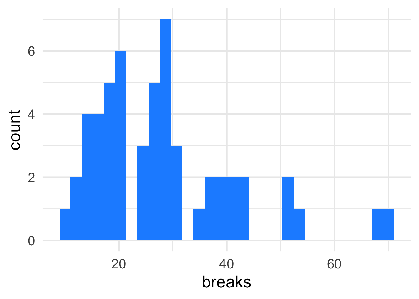
We can look at the distribution of breaks in the data
The variance is much greater than the mean, which suggests that we will have over-dispersion in the model.
9.2 Fit Poisson model
We fit a Poisson linear model to model the number of breaks as a function of the predictors wool and tension.
fit3 <-glm(breaks ~ wool+tension, data=warpbreaks, family ="poisson")summary(fit3)
Call:
glm(formula = breaks ~ wool + tension, family = "poisson", data = warpbreaks)

Coefficients:
            Estimate Std. Error z value Pr(>|z|)
(Intercept)  3.69196    0.04541  81.302  < 2e-16 ***
woolB       -0.20599    0.05157  -3.994 6.49e-05 ***
tensionM    -0.32132    0.06027  -5.332 9.73e-08 ***
tensionH    -0.51849    0.06396  -8.107 5.21e-16 ***
---
Signif. codes:  0 '***' 0.001 '**' 0.01 '*' 0.05 '.' 0.1 ' ' 1

(Dispersion parameter for poisson family taken to be 1)

    Null deviance: 297.37  on 53  degrees of freedom
Residual deviance: 210.39  on 50  degrees of freedom
AIC: 493.06

Number of Fisher Scoring iterations: 4
Exercise
What do these results tell you?
9.3 Model selection
Is the inclusion of the levels of tension informative or not? Which model is better, with or without such variable?
To test for the global significance of the tension variable, we can fit a model without it and perform an Analysis of Deviance (likelihood ratio test) comparing a Poisson GLM with and without the tension variable
fit4 <-glm(breaks ~ wool, data=warpbreaks, family ="poisson")summary(fit4)
Call:
glm(formula = breaks ~ wool, family = "poisson", data = warpbreaks)

Coefficients:
            Estimate Std. Error z value Pr(>|z|)
(Intercept)  3.43518    0.03454  99.443  < 2e-16 ***
woolB       -0.20599    0.05157  -3.994 6.49e-05 ***
---
Signif. codes:  0 '***' 0.001 '**' 0.01 '*' 0.05 '.' 0.1 ' ' 1

(Dispersion parameter for poisson family taken to be 1)

    Null deviance: 297.37  on 53  degrees of freedom
Residual deviance: 281.33  on 52  degrees of freedom
AIC: 560

Number of Fisher Scoring iterations: 4
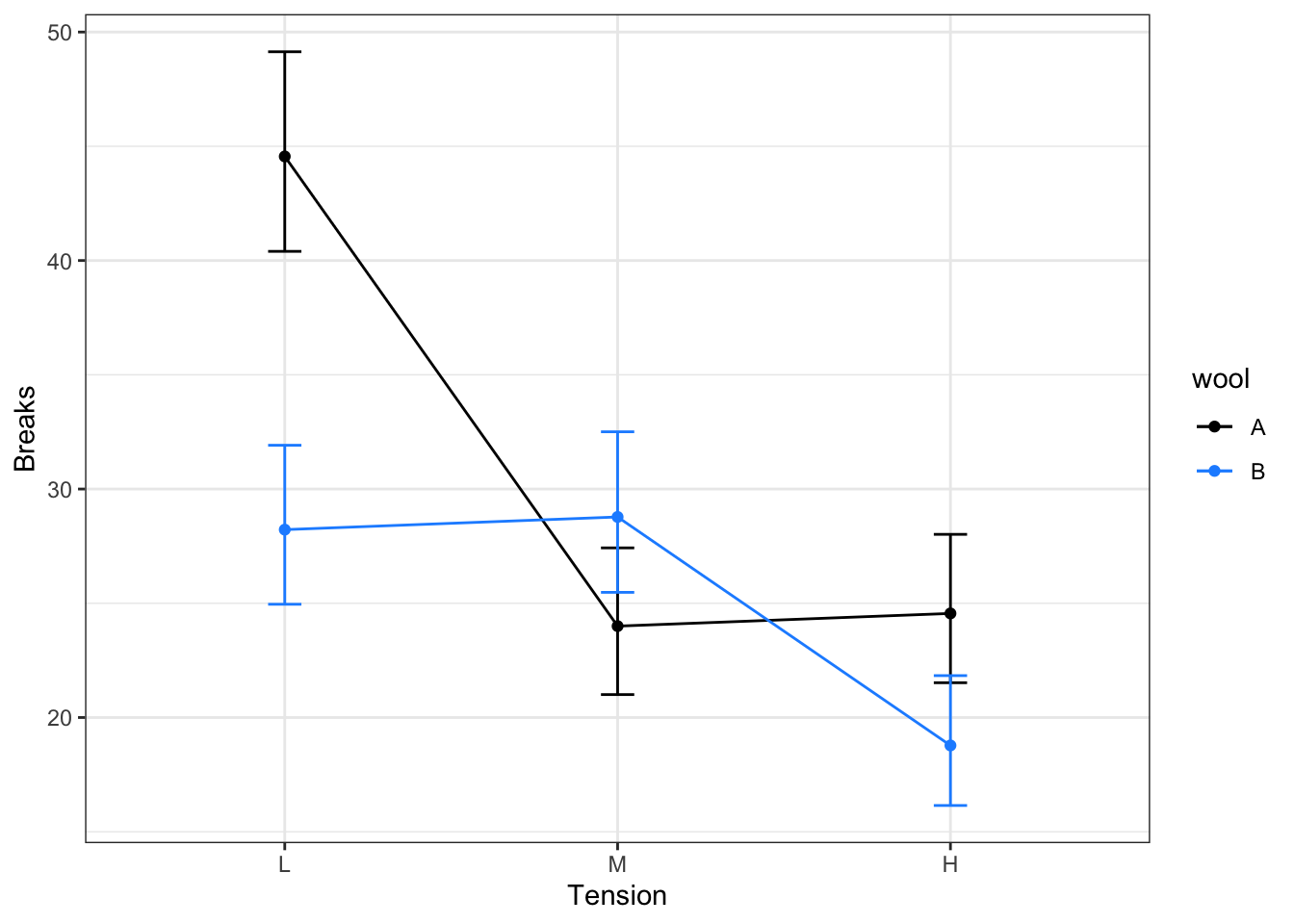
The p value is really small, it means that the interaction is significant, i.e., the difference in the number of breaks between wool types changes across tension levels.
Note
If interaction is significant, Do not interpret main effects alone. Interpret how the effect of one variable changes across levels of the other variable.
Effects of interest = linear combinations of main + interaction terms.
The \(DI= 3.8 >2\), this indicates strong overdispersion. Hence, the Poisson model is underestimating the variability in the data, and a diffent approach maybe necessary. A common solution could be, consider the negative binomial model.
# A tibble: 6 × 6
  Enrollment type     nv nvrate enroll1000 region
       <dbl> <chr> <dbl>  <dbl>      <dbl> <chr>
1       5590 U        30 5.37         5.59 SE
2        540 C         0 0            0.54 SE
3      35747 U        23 0.643       35.7  W
4      28176 C         1 0.0355      28.2  W
5      10568 U         1 0.0946      10.6  SW
6       3127 U         0 0            3.13 SW
The goal is to study whether is an association among the number of violent crimes, region and the type of school.
10.1 Data wrangling and exploration
We combine the SW and SE to form a single category of the South because Southwestern colleges has 0 observed rate.
c_data <- c_data %>%mutate(region2 =case_when( region %in%c("SW", "SE") ~"S",TRUE~ region ))
We then turn the categorical variables into factors.
# A tibble: 6 × 7
  Enrollment type     nv nvrate enroll1000 region region2
       <dbl> <fct> <dbl>  <dbl>      <dbl> <chr>  <fct>
1       5590 U        30 5.37         5.59 SE     S
2        540 C         0 0            0.54 SE     S
3      35747 U        23 0.643       35.7  W      W
4      28176 C         1 0.0355      28.2  W      W
5      10568 U         1 0.0946      10.6  SW     S
6       3127 U         0 0            3.13 SW     S
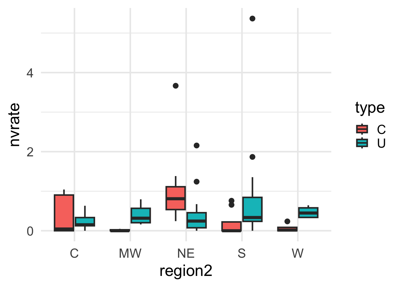
We can now look at the number of crimes across the type of schools and regions.
In general the mean violent crime rates of universities is lower than the mean violent crime rates of colleges within a region (except the Northeast).
The regional pattern of rates at universities appears to differ from that of the colleges across different regions.
There are several outliers.
We filter out the outliers
c_data_filt<- c_data %>%filter(nvrate <=2)
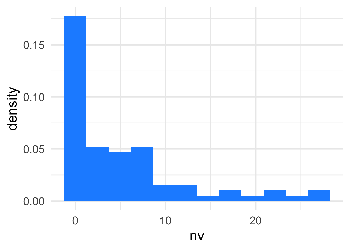
Plot the density of violent crime rates
ggplot(c_data_filt, aes(x=nv)) +geom_histogram(aes(y =after_stat(density)), fill ="dodgerblue", bins =12)
From the histogram plot, we can see many schools reported few crimes, and a few schools have a large number of crimes. Moreover, the shape of the density does not look like a normal distribution. Therefore, Poisson regression should be considered to model the data.
10.2 Fit Poisson linear models
It is also important to note that the counts are not directly comparable because they come from different school size. We expect schools with more students to have more reports of violent crime since there are more students who could be affected. Therefore, we take the differences in enrollments into account by including an offset in our model, i.e., consider a Poisson regression of the form \[\log(\frac{\lambda}{\text{enroll1000}})=\beta_0+\beta_1 \text{type}\] or \[\log(\lambda)=\beta_0+\beta_1 \text{type}+\log(\text{enroll1000})\]
fit7 <-glm(nv ~ type + region2, family ="poisson", offset=log(enroll1000), data=c_data_filt)summary(fit7)
Call:
glm(formula = nv ~ type + region2, family = "poisson", data = c_data_filt,
    offset = log(enroll1000))

Coefficients:
            Estimate Std. Error z value Pr(>|z|)
(Intercept)  -1.7969     0.1870  -9.611  < 2e-16 ***
typeU         0.5567     0.1536   3.625 0.000289 ***
region2MW     0.1004     0.1775   0.565 0.571763
region2NE     0.5663     0.1607   3.524 0.000425 ***
region2S      0.5836     0.1490   3.918 8.94e-05 ***
region2W      0.3077     0.1874   1.641 0.100701
---
Signif. codes:  0 '***' 0.001 '**' 0.01 '*' 0.05 '.' 0.1 ' ' 1

(Dispersion parameter for poisson family taken to be 1)

    Null deviance: 323.91  on 77  degrees of freedom
Residual deviance: 283.86  on 72  degrees of freedom
AIC: 499.55

Number of Fisher Scoring iterations: 5
These results tell us the Northeast and the South differ significantly from the Central region. The estimated coefficient of 0.5663 means that the violent crime rate per 1000 in the Northeast is 1.76 ( \(=\exp( 0.5663)\)) times that of the Central region when the type of school is the same.
Exercise
Fit the Poisson linear model on the original data (without filtering out outliers). What do you notice?
We also note that the effect of the type may vary denpending on the region, so we also consider a Poisson regression model with interaction between type and region.
fit8 <-glm(nv ~ type * region2, family ="poisson", offset =log(enroll1000), data = c_data_filt)summary(fit8)
Call:
glm(formula = nv ~ type * region2, family = "poisson", data = c_data_filt,
    offset = log(enroll1000))

Coefficients:
                Estimate Std. Error z value Pr(>|z|)
(Intercept)      -1.4741     0.3536  -4.169 3.05e-05 ***
typeU             0.1959     0.3775   0.519  0.60377
region2MW        -1.9765     1.0607  -1.863  0.06239 .
region2NE         1.1732     0.3994   2.938  0.00331 **
region2S         -0.1562     0.4859  -0.322  0.74779
region2W         -1.8337     0.7906  -2.319  0.02037 *
typeU:region2MW   2.1965     1.0765   2.040  0.04132 *
typeU:region2NE  -0.8016     0.4381  -1.830  0.06732 .
typeU:region2S    0.8121     0.5108   1.590  0.11185
typeU:region2W    2.4106     0.8140   2.962  0.00306 **
---
Signif. codes:  0 '***' 0.001 '**' 0.01 '*' 0.05 '.' 0.1 ' ' 1

(Dispersion parameter for poisson family taken to be 1)

    Null deviance: 323.91  on 77  degrees of freedom
Residual deviance: 236.02  on 68  degrees of freedom
AIC: 459.7

Number of Fisher Scoring iterations: 6
Exercise
What do these results tell you?
These results confirm the significance of the interaction between the effect of region and the type of institution. We also can perform a test to see where the interaction is significant.
anova(fit7, fit8)
Analysis of Deviance Table

Model 1: nv ~ type + region2
Model 2: nv ~ type * region2
  Resid. Df Resid. Dev Df Deviance  Pr(>Chi)
1        72     283.86
2        68     236.02  4   47.841 1.018e-09 ***
---
Signif. codes:  0 '***' 0.001 '**' 0.01 '*' 0.05 '.' 0.1 ' ' 1
10.3 Check overdispersion
The dispersion index is
DI =236.02/68DI
[1] 3.470882
The \(DI= 3.47 >2\), this indicates there exist strong overdispersion. Hence, a different approach is neccessary!!
10.4 Further reading
S. Holmes and W. Huber. Modern Statistics for Modern Biology. Chapter 8.