Generalized Linear Models
Advanced Statistics and Data Analysis
Introduction
Linear models
Linear models are the most useful applied statistics technique.
However, they have their limitations:
- The response may not be continuous
- The response may have a limited range of possible values
In such cases, linear models are not ideal and we may want to consider generalizations of it.
Generalized Linear Models (GLMs)
The Generalized Linear Model (GLM) is a family of models that includes the linear model and extend it to situations in which the response variable has a distribution of the exponential family.
The exponential family is a family of distributions that includes the Gaussian, Poisson, Binomial, Gamma, among others.
Exponential Family
The density function of a distribution of the exponential family can be written as \[ f(y_i; \theta_i, \phi) = \exp \left\{\frac{y_i \theta_i - b(\theta_i)}{a(\phi)} + c(y_i, \phi)\right\}, \] where:
- \(\theta_i\) are the canonical parameters;
- \(\phi\) is the dispersion parameter;
- \(a\), \(b\), and \(c\) are functions that depend on the specific distribution.
Example: Poisson distribution
The probability function of a Poisson distribution can be written as \[ f(y_i; \lambda_i) = \frac{\lambda_i^{y_i} e^{-\lambda_i}}{y_i!}, \]
or equivalently as \[ f(y_i; \lambda_i) = \exp\left\{y_i \log(\lambda_i) - \lambda_i - \log(y_i!)\right\}, \]
which corresponds to an exponential family with:
- \(\theta_i = \log(\lambda_i)\);
- \(b(\theta_i) = \exp(\theta_i)\);
- \(a(\phi) = 1\);
- \(c(y_i, \phi) = -\log(y_i!)\).
Log-likelihood function
Note that the log-likelihood function of the exponential family can be written as \[ \ell(\lambda; y) = \sum_{i=1}^n \frac{y_i \theta_i - b(\theta_i)}{a(\phi)} + c(y_i, \phi). \]
One can show that: \[ E[Y_i] = \mu_i = b'(\theta_i) \] and \[ Var(Y_i) = b''(\theta_i) a(\phi), \]
where \(b'()\) and \(b''()\) are the first and second derivative of \(b\).
Important
Note that the variance depends on the mean!
Example: Poisson distribution
In the case of the Poisson, \(b(\theta_i) = \exp(\theta_i)\) and \(a(\phi) = 1\), hence:
\[ E[Y_i] = \exp(\theta_i) = \lambda_i \] and
\[ Var(Y_i) = \exp(\theta_i) = \lambda_i. \]
Generalizations of the linear model
We can think of GLMs as a two-way generalization of linear models:
We can use a function of the linear predictor to transform it to a range of values that is more useful for the application.
We can use a different distribution for the error terms other than the Gaussian.
Likelihood estimation
Recall that ordinary least squares can be seen as the maximum likelihood estimate of the linear regression parameters.
The idea is that by changing the distribution of the response variable, we can still use maximum likelihood to estimate the regression coefficients, but specifying a different likelihood function.
The three components of a GLM
The three components that we need in order to fully specify a GLM are:
An exponential family distribution for the response.
A link function that connects the linear predictor to the response.
A variance function that specifies how the variance depends on the mean.
Example: the normal linear model
If we assume that:
The response variable is distributed as a Gaussian r.v.
The link function is the identity function.
The variance is constant with respect to the mean.
Then, we have the standard linear model.
Example: the normal linear model
In formulas:
\(Y \sim \mathcal{N}( \mu, \sigma^2)\).
\(E[Y | X] = X \beta\).
\(V(\mu) = \sigma^2\).
Example: logistic regression
Logistic regression assumes that:
The response variable is distributed as a Bernoulli r.v.
The link function is the logistic function.
The variance is a function of the mean.
Example: logistic regression
In formulas:
\(Y \sim \mathcal{Be}(\mu)\).
\(g(E[Y | X]) = X \beta\), where \(g(\mu) = \log \left(\frac{\mu}{1-\mu}\right)\).
\(V(\mu) = \mu (1 - \mu)\).
Note that the link function implies that \[ \mu = \frac{\exp(X \beta)}{1 + \exp(X\beta)}. \]
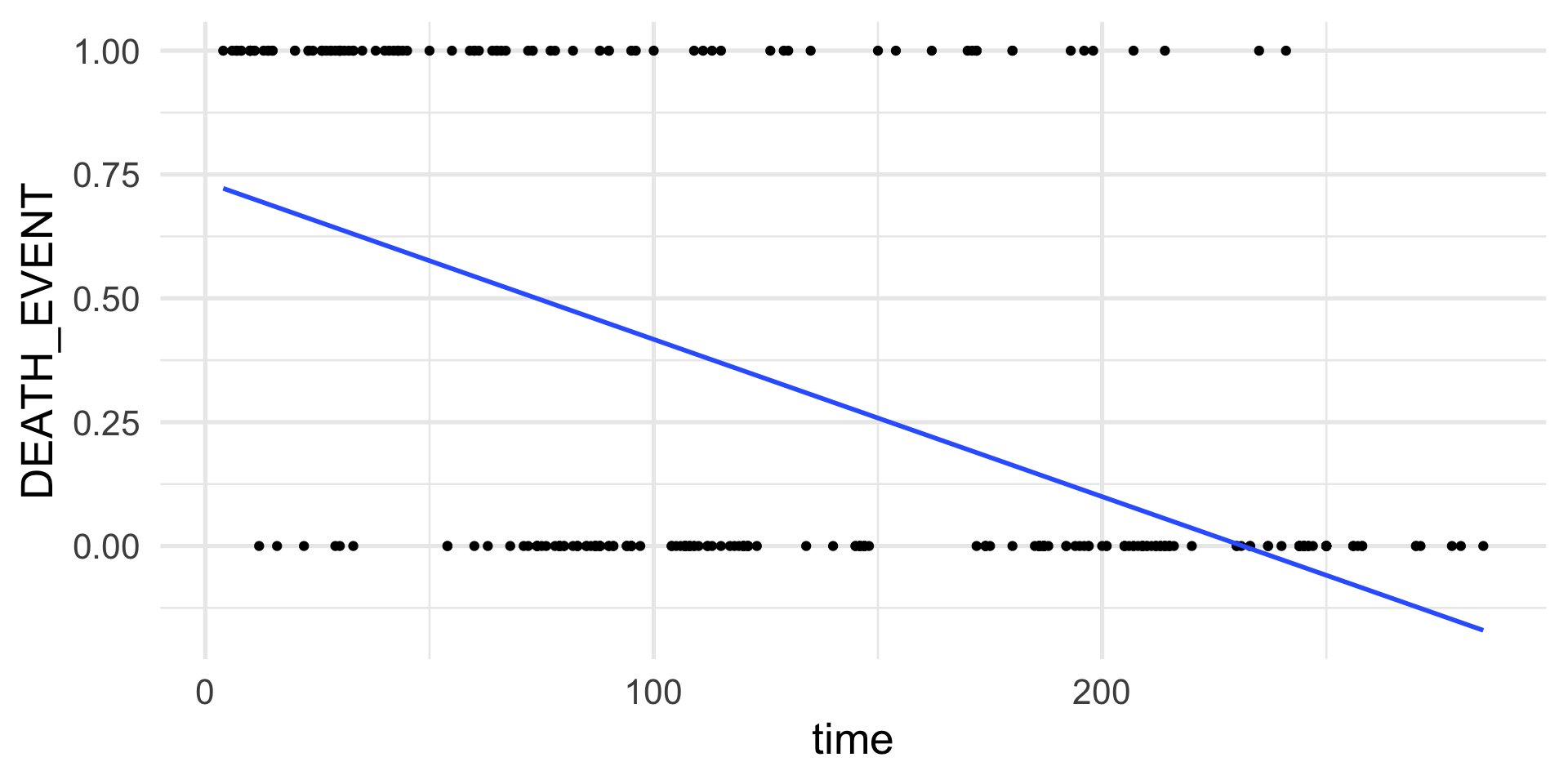
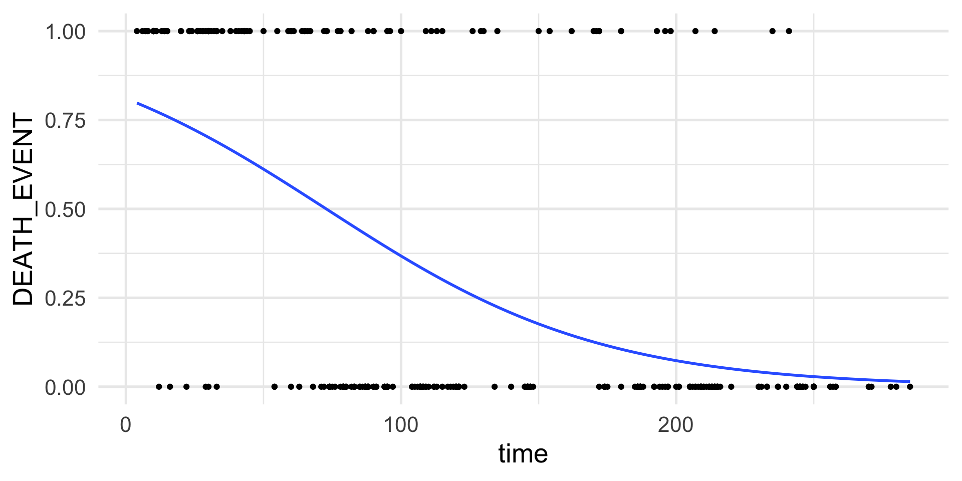
Example: logistic regression
Assume that we have collected data from 299 patients that had heart failure.
For each patient we measure if they died or survived after a follow-up period.
We can use a set of 13 clinical features to try to predict patient survival.
- In total, 96 patients out of 299 died.
Example: logistic regression
Example: logistic regression
Example: Poisson regression
Poisson regression (or log-linear regression) assumes that:
The response variable is distributed as a Poisson r.v.
The link function is the log function.
The variance is a function of the mean.
Example: Poisson regression
In formulas:
\(Y \sim \mathcal{Poi}(\mu)\).
\(g(E[Y | X]) = X \beta\), where \(g(\mu) = \log(\mu)\).
\(V(\mu) = \mu\).
Note that the link function implies that \[ \mu = \exp(X \beta) \]
The log is called the canonical link function because it is equal to the function that transforms the mean into the canonical parameter in the exponential family formulation.
Example: Poisson regression
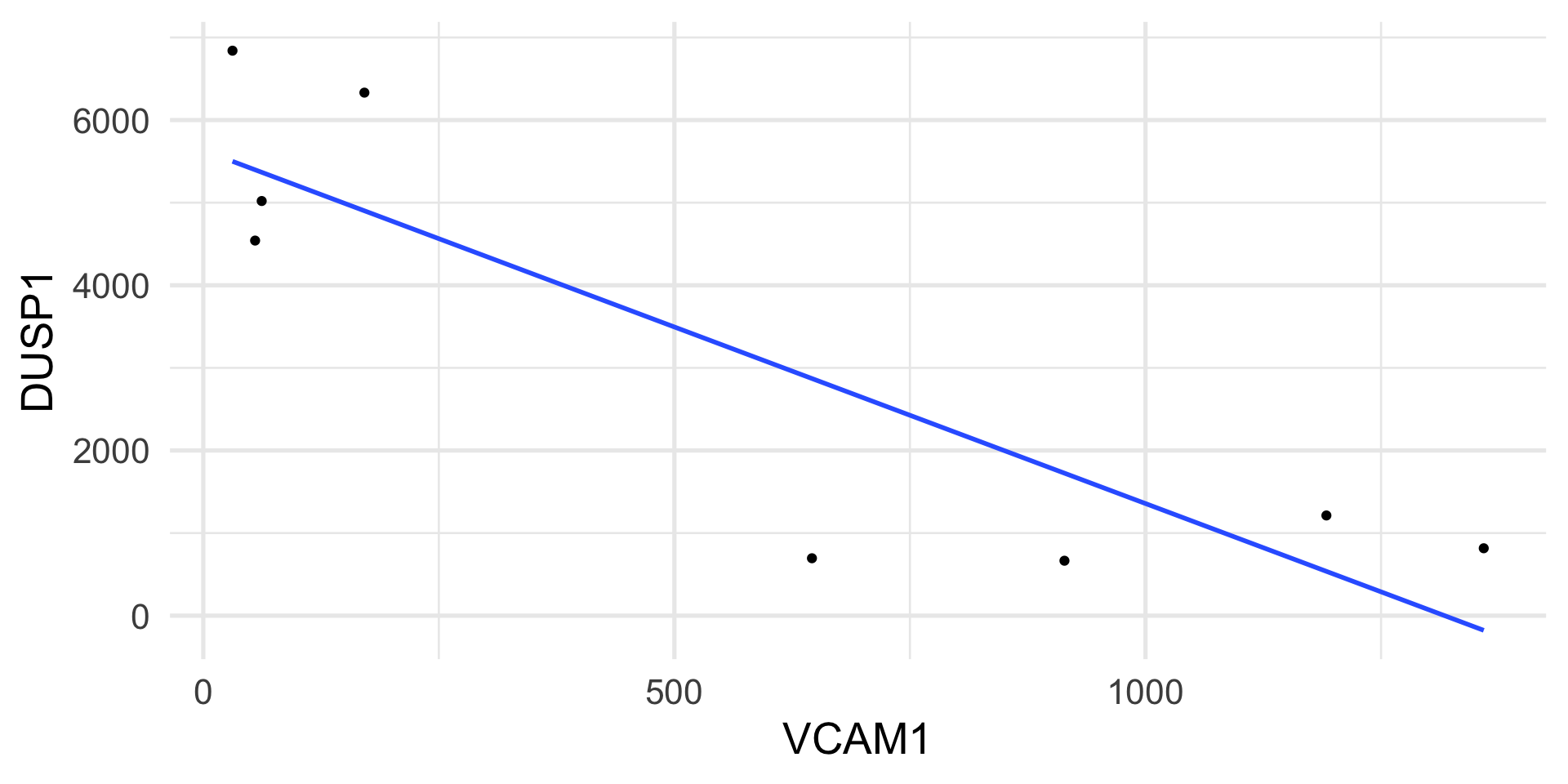
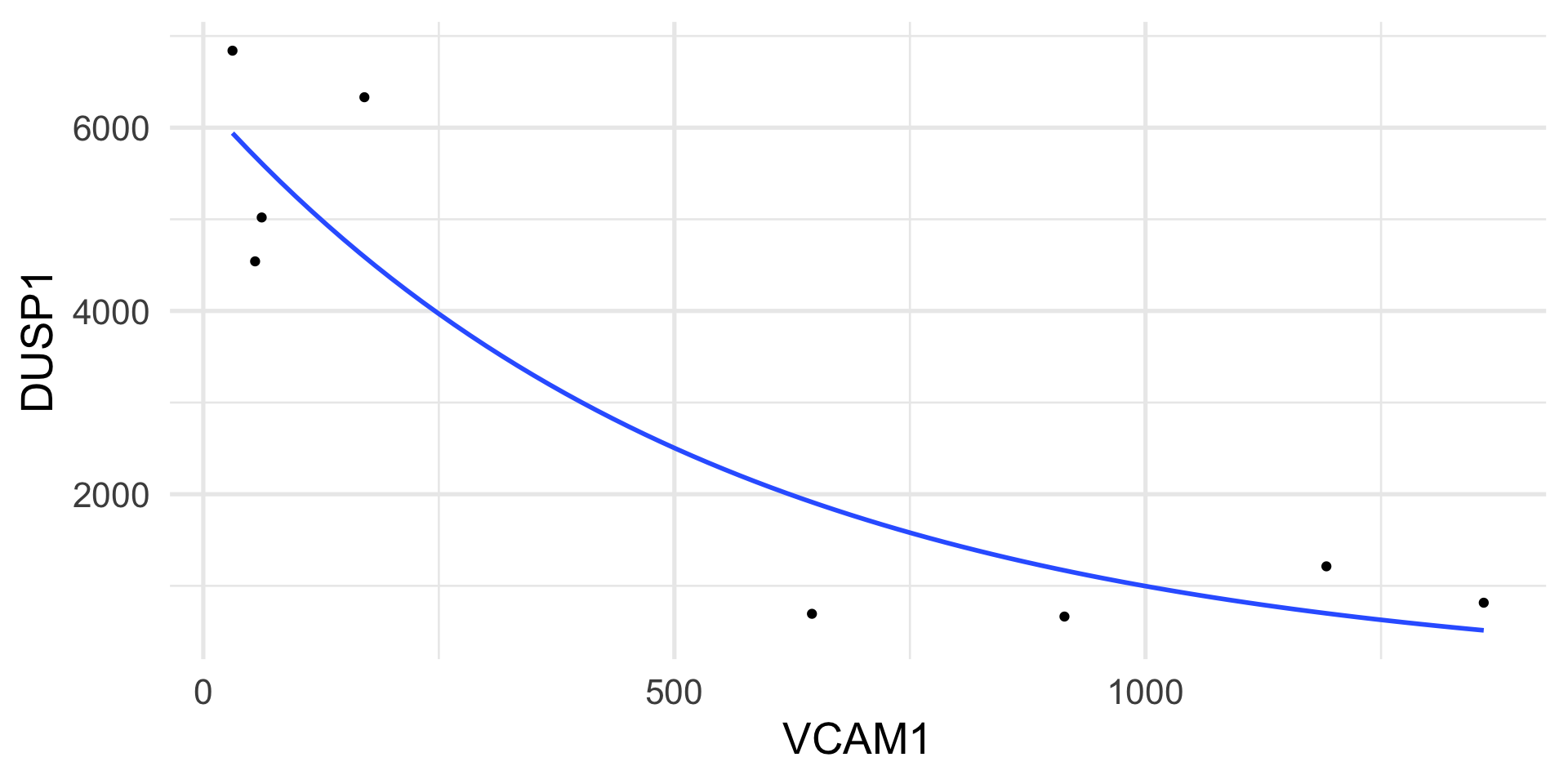
We measure the expression of two genes, DUSP1 and VCAM1, in airway smooth muscle (ASM) cell lines.
The DUSP1 gene plays an important role in the human cellular response to environmental stress.
The VCAM1 gene is involved in cell adhesion and signal transduction.
The genes are measured with an assay that yields counts as a measure of gene expression.
Example: Poisson regression
Example: Poisson regression
Parameter estimation
Log-likelihood of a GLM
In principle, we can maximize the log-likelihood as a function of the regression coefficients.
In fact, once we have defined a relationship between the parameter of the model and the predictors, we can write the likelihood as a function of \(\beta\).
In the case of the Poisson, the log-likelihood is \[ \ell(\beta; X, y) = \sum_{i=1}^n y_i \eta_i- \exp\{\eta_i\}, \] where \(\eta_i = \log(\mu_i) = \sum_{k=1}^p x_{ik} \beta_k\).
Score function
The derivative of the log-likelihood with respect to \(\theta\) is also called the score function.
One can show that in the exponential family, the score function \[ S(\theta) = \sum_{i=1}^n \frac{y_i - \mu_i}{a(\phi)}, \]
when you want to derive for \(\beta\), the chain rule of differentiation gives \[ S(\beta) = \sum_{i=1}^n \frac{Y_i - \mu_i}{Var(Y_i)} \frac{d \mu_i}{d \eta_i} X^\top = X^\top A (Y - \mu), \]
where \(A\) is a diagonal matrix with elements \(a_{ii} = (Var(Y_i) \frac{d \eta_i}{d \mu_i})^{-1}\).
Important
Note the relation with least squares!
Poisson example
In Poisson data:
- \(Var(Y_i) = E[Y_i] = \mu_i\);
- \(\eta_i = \log(\mu_i)\), hence \(\frac{d \eta_i}{d \mu_i} = \frac{1}{\mu_i}\).
Hence, \(A = I\), the identity matrix and \[ S(\beta) = X^\top (Y - \mu). \]
Solving the score equations
To find the MLE we need to solve the equation \[ S(\beta) = X^\top A (Y - \mu) = 0. \]
The problem is that this is non linear in \(\beta\) because of the link function.
We hence need numerical algorithms to find the values of \(\beta\) that solve this equation.
Newton-Raphson
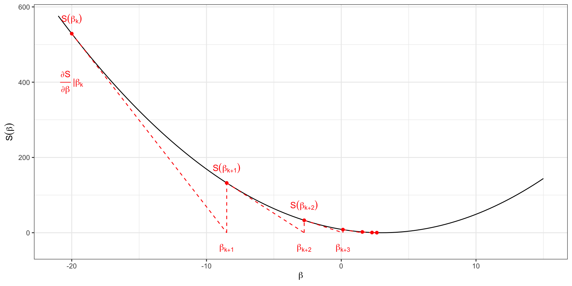
Newton-Raphson
The Newton-Raphson algorithm is a numerical algorithm to find the “root” of a function, i.e., to find the value for which that function is equal to 0.
It starts from an initial guess, say \(\beta_k\), and moves in the direction of the derivative until it intersects the zero line.
Newton-Raphson
Specifically:
- Choose an initial parameter estimate \(\beta_k\);
- Calculate the score \(S(\beta_k)\);
- Calculate the derivative \(\frac{\partial S(\beta)}{\partial \beta}\) at the value \(\beta_k\);
- Go in the direction of the derivative until the point, \(\beta_{k+1}\) in which it crosses the zero line;
- Update the value of \(\beta\) to \(\beta_{k+1}\);
- Iterate 2-5 until convergence.
Derivative of the score
For the Newton-Raphson algorithm to work, we need to compute the derivative of the score function.
One can show that it is \[ \frac{\partial S(\beta)}{\partial \beta} = - X^\top W X, \] where \(W\) is a diagonal matrix with elements \[ w_{ii} = \frac{(d \mu_i / d \eta_i)^2}{Var(Y_i)} \]
Iteratively Reweighted Least Squares
Now that we know the derivative, we can rewrite the Newton-Raphson algorithm as the Iteratively Reweighted Least Squares (IRLS).
In fact we can show that \[ \beta_{k+1} = \beta_k + (X^\top W X)^{-1} S(\beta_k) \] or equivalently \[ \beta_{k+1} = (X^\top W X)^{-1} X^\top W Z, \] where \[ Z = X \beta_k + \frac{\partial \eta}{\partial \mu} (Y - \mu). \]
Interpretation of IRLS
Note that the estimate of \(\beta\) at iteration \(k\) is similar to the least squares estimator, but it is weighted by a function of the variance.
This is a way to account for the heteroschedasticity of the data.
In R: the glm() function
In R there is a very convenient function that implements the IRLS algorithm and has a syntax very similar to the lm() function.
In addition to the formula, you need to specify the family of distributions you want to specify for the response variable and (implicitly or explicitly) the link function.
Example: Poisson regression
In the airway smooth muscle (ASM) cell lines, we have two additional variables to consider:
The cell lines were either untreated or treated with dexamethasone (
dex).The cell lines were derived from four distinct donors (
cell).
It is of interest to check whether the DUSP1 gene changes between treated and control cells, potentially accounting for the differences in cell lines.
Example: Poisson regression
Call:  glm(formula = DUSP1 ~ dex, family = poisson, data = df)

Coefficients:
(Intercept)       dextrt
      6.742        1.903

Degrees of Freedom: 7 Total (i.e. Null);  6 Residual
Null Deviance:      16880
Residual Deviance: 831.4    AIC: 911.5
Interpretation of the parameters
The Poisson regression model can be written as \[ \log \mu_i = \beta_0 + \beta_1 x_{i}, \] where \(x_i=1\) if the cells are treated and \(x_i=0\) if untreated.
Hence, \[ \log(\mu_i | x_i = 1) - \log(\mu_i | x_i = 0) = \beta_1 \]
which leads to \[ \beta_1 = \log \left(\frac{\mu_i | x_i = 1}{\mu_i | x_i = 0}\right). \]
Example: logistic regression
In the heart failure dataset, we may be interested in the relation between diabetes and heart failure.
Example: logistic regression
Call:  glm(formula = DEATH_EVENT ~ diabetes, family = binomial, data = heart)

Coefficients:
(Intercept)     diabetes
  -0.745333    -0.008439

Degrees of Freedom: 298 Total (i.e. Null);  297 Residual
Null Deviance:      375.3
Residual Deviance: 375.3    AIC: 379.3
Interpretation of the parameters
The logistic regression model can be written as \[ \log \left( \frac{\mu_i}{1-\mu_i} \right)= \beta_0 + \beta_1 x_{i}, \] where \(x_i=1\) if the subject has diabetes and \(x_i=0\) if not.
Hence, \[ \log \left( \frac{\mu_1}{1-\mu_1} \right) - \log \left( \frac{\mu_0}{1-\mu_0} \right) = \beta_1, \] where we indicate with \(\mu_1 = E[Y|x=1]\) and \(\mu_0 = E[Y|x=0]\).
We can thus interpret \(\beta_1\) as the log odds ratio \[ \beta_1 = \log OR = \log \left(\frac{\mu_1 / (1-\mu_1)}{\mu_0 / (1-\mu_0)}\right). \]
Inference
Likelihood Ratio Test
The analogous of the sum of squares and the F test in GLMs is the log-likelihood and the likelihood ratio test.
We can use the likelihood to compare two models, as we have done with the F statistics in linear models.
One can show that, when \(n \to \infty\), \[ D = 2 [\ell(\hat\beta) - \ell(\hat\beta^0)] \stackrel{H_0}{\sim} \chi^2_{df-df_0}, \]
where \(\hat\beta\) and \(\hat\beta^0\) are the estimates of the coefficient under the full and reduced model, with \(df\) and \(df_0\) degrees of freedom, respectively.
Wald Test
An alternative to the LRT is the Wald test, that leverages the fact that when \(n \to \infty\), \[ \hat\beta \stackrel{H_0}{\sim} \mathcal{N}(\beta, (X^\top W X)^{-1}). \]
Hence, the statistic \[ t = \frac{\hat\beta_k}{\sqrt{[(X^\top W X)^{-1}]_{kk}}} \stackrel{H_0}{\sim} N(0, 1) \] can be used to compute confidence intervals and test the null hypothesis \(\beta_k = 0\).
Example: Poisson regression
In the airway smooth muscle (ASM) cell lines, we have two additional variables to consider:
The cell lines were either untreated or treated with dexamethasone (
dex).The cell lines were derived from four distinct donors (
cell).
It is of interest to check whether the DUSP1 gene changes between treated and control cells, potentially accounting for the differences in cell lines.
Poisson regression: Wald test
Call:
glm(formula = DUSP1 ~ dex, family = poisson, data = df)

Coefficients:
            Estimate Std. Error z value Pr(>|z|)
(Intercept)  6.74200    0.01718   392.5   <2e-16 ***
dextrt       1.90328    0.01841   103.4   <2e-16 ***
---
Signif. codes:  0 '***' 0.001 '**' 0.01 '*' 0.05 '.' 0.1 ' ' 1

(Dispersion parameter for poisson family taken to be 1)

    Null deviance: 16883.9  on 7  degrees of freedom
Residual deviance:   831.4  on 6  degrees of freedom
AIC: 911.48

Number of Fisher Scoring iterations: 4
Poisson regression: Wald Test
Call:
glm(formula = DUSP1 ~ dex + cell, family = poisson, data = df)

Coefficients:
            Estimate Std. Error z value Pr(>|z|)
(Intercept)  6.61541    0.02075 318.808   <2e-16 ***
dextrt       1.90328    0.01841 103.363   <2e-16 ***
cellN061011  0.26966    0.01751  15.403   <2e-16 ***
cellN080611  0.21694    0.01771  12.249   <2e-16 ***
cellN61311  -0.01206    0.01870  -0.645    0.519
---
Signif. codes:  0 '***' 0.001 '**' 0.01 '*' 0.05 '.' 0.1 ' ' 1

(Dispersion parameter for poisson family taken to be 1)

    Null deviance: 16883.90  on 7  degrees of freedom
Residual deviance:   416.88  on 3  degrees of freedom
AIC: 502.96

Number of Fisher Scoring iterations: 4
Poisson regression: LRT
Analysis of Deviance Table

Model 1: DUSP1 ~ dex
Model 2: DUSP1 ~ dex + cell
  Resid. Df Resid. Dev Df Deviance  Pr(>Chi)
1         6     831.40
2         3     416.88  3   414.52 < 2.2e-16 ***
---
Signif. codes:  0 '***' 0.001 '**' 0.01 '*' 0.05 '.' 0.1 ' ' 1
Logistic regression:
Call:
glm(formula = DEATH_EVENT ~ . - time, family = binomial, data = heart)

Coefficients:
                           Estimate Std. Error z value Pr(>|z|)
(Intercept)               4.964e+00  4.601e+00   1.079 0.280625
age                       5.569e-02  1.313e-02   4.241 2.23e-05 ***
anaemia                   4.179e-01  3.009e-01   1.389 0.164904
creatinine_phosphokinase  2.905e-04  1.428e-04   2.034 0.041907 *
diabetes                  1.514e-01  2.974e-01   0.509 0.610644
ejection_fraction        -7.032e-02  1.486e-02  -4.731 2.23e-06 ***
high_blood_pressure       4.189e-01  3.061e-01   1.369 0.171092
platelets                -7.094e-07  1.617e-06  -0.439 0.660857
serum_creatinine          6.619e-01  1.734e-01   3.817 0.000135 ***
serum_sodium             -5.667e-02  3.338e-02  -1.698 0.089558 .
sex                      -3.990e-01  3.508e-01  -1.137 0.255394
smoking                   1.356e-01  3.486e-01   0.389 0.697300
---
Signif. codes:  0 '***' 0.001 '**' 0.01 '*' 0.05 '.' 0.1 ' ' 1

(Dispersion parameter for binomial family taken to be 1)

    Null deviance: 375.35  on 298  degrees of freedom
Residual deviance: 294.28  on 287  degrees of freedom
AIC: 318.28

Number of Fisher Scoring iterations: 5
Logistic regression: Wald test
Analysis of Deviance Table

Model 1: DEATH_EVENT ~ age + sex + smoking
Model 2: DEATH_EVENT ~ (age + anaemia + creatinine_phosphokinase + diabetes +
    ejection_fraction + high_blood_pressure + platelets + serum_creatinine +
    serum_sodium + sex + smoking + time) - time
  Resid. Df Resid. Dev Df Deviance  Pr(>Chi)
1       295     355.82
2       287     294.28  8   61.536 2.327e-10 ***
---
Signif. codes:  0 '***' 0.001 '**' 0.01 '*' 0.05 '.' 0.1 ' ' 1