Differential Expression Analysis
Source:vignettes/differential_expression.Rmd
differential_expression.RmdLoad data and filtering
We start by loading the airway data and repeat the same gene filter that we applied in the previous vignette.
data(airway)

filter <- filterByExpr(airway)
## Warning in filterByExpr.DGEList(y, design = design, group = group, lib.size =
## lib.size, : All samples appear to belong to the same group.
table(filter)## filter
## FALSE TRUE
## 49453 14224
filtered <- airway[filter,]

filtered
## class: RangedSummarizedExperiment
## dim: 14224 8
## metadata(1): ''
## assays(1): counts
## rownames(14224): ENSG00000000003 ENSG00000000419 ... ENSG00000273382
## ENSG00000273486
## rowData names(10): gene_id gene_name ... seq_coord_system symbol
## colnames(8): SRR1039508 SRR1039509 ... SRR1039520 SRR1039521
## colData names(9): SampleName cell ... Sample BioSampleNow we can create a DESEqDataSet object: this is the
object that we will use to conduct our differential expression
analysis.
Note that we start from the SummarizedExperiment object
and we add a design matrix that specifies which columns of the
colData we will use as covariates in the statistical
model.
dds <- DESeqDataSet(filtered,
                    design = ~ cell + dex)
dds
## class: DESeqDataSet
## dim: 14224 8
## metadata(2): '' version
## assays(1): counts
## rownames(14224): ENSG00000000003 ENSG00000000419 ... ENSG00000273382
## ENSG00000273486
## rowData names(10): gene_id gene_name ... seq_coord_system symbol
## colnames(8): SRR1039508 SRR1039509 ... SRR1039520 SRR1039521
## colData names(9): SampleName cell ... Sample BioSampleNote that the DESeqDataSet class “inherits” from SummarizedExperiment, meaning that an object of this class is also a SummarizedExperiment and all its methods are still applicable.
class(dds)## [1] "DESeqDataSet"
## attr(,"package")
## [1] "DESeq2"
is(dds, "SummarizedExperiment")## [1] TRUECount-based differential expression
The DESeq2 package (as well as edgeR the
other popular package for differential expression) uses a strategy that
models the RNA-seq read counts directly in a Negative Binomial
Generalized Linear Model (GLM).
Hence, unlike other approaches, we will apply our statistical model directly to the count data, without the need for data transformation.
In particular, for each gene, we fit a GLM with the formula specified
above and we test the null hypothesis \[
H_0: \beta = 0
\] against a bilateral alternative, where \(\beta\) is the coefficient of the covariate
that we want to test (to be specified later), in this case
dex, the treatment.
Normalization
What we discussed about normalization is still relevant: we do not want to misinterpret technical differences as biological ones and identify genes that appear to differ between treated and control samples only because of technical reason.
However, transforming the data via normalization is not an option since we want our GLM to model count data. The solution is to estimate the size factors and include them in the model as offsets.
dds <- estimateSizeFactors(dds)

ggplot(data.frame(libSize = apply(assay(dds), 2, quantile, .75),
                  sizeFactor = sizeFactors(dds),
                  Group = dds$cell),
       aes(x = libSize, y = sizeFactor, col = Group)) +
    geom_point(size = 3)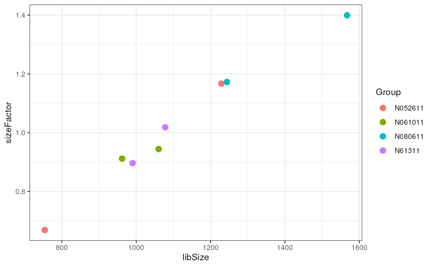
Dispersion Estimation
Usually, the Poisson distribution is a good starting point for count data. However, RNA-seq data are overdispersed, meaning that the variance is greater than the mean.
For this reason, DESeq2 and edgeR use a negative binomial that assumes that the variance is a quadratic function of the mean:
\[ V(\mu) = \mu + \phi \mu^2, \] where \(\phi\) is the dispersion parameter, to be estimated for each gene.
Since we tipically have very large \(p\) (genes) and small-ish \(n\) (samples), a good strategy is to “borrow strength” across genes to improve the accuracy in the estimation of the dispersion parameters.
DESeq2’s strategy is to first compute a preliminary genewise estimate
via maximum likelihood estimation, then estimate the mean-dispersion
relationship fitting a regression line and finally shrinking
the estimates towards the fit. All three steps are performed within the
estimateDispersions function.
dds <- estimateDispersions(dds)## gene-wise dispersion estimates## mean-dispersion relationship## final dispersion estimates
plotDispEsts(dds)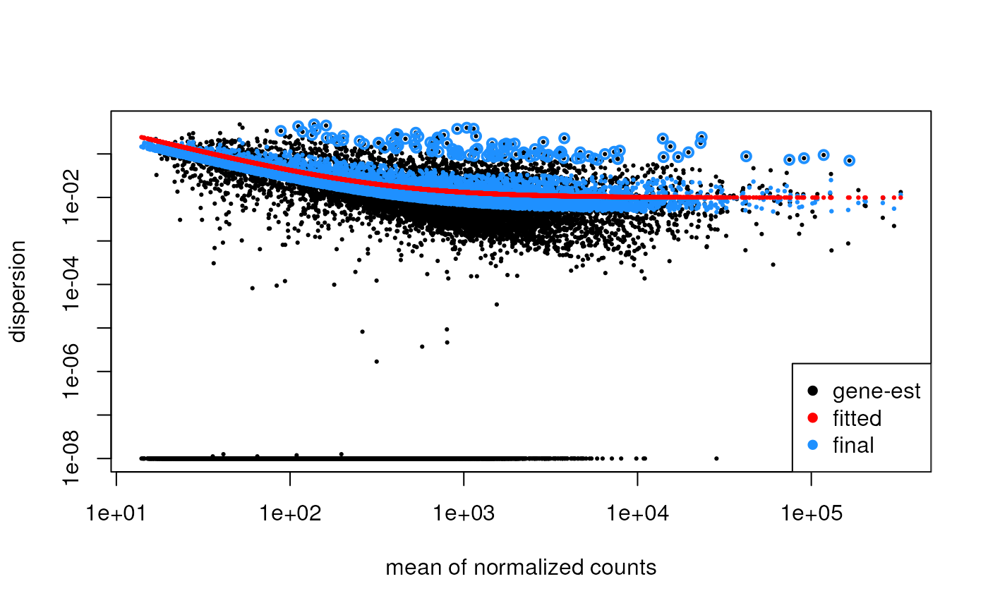
Test for DE
Finally, we can use a Wald test to test the differential expression between, say, treated and control.
dds <- nbinomWaldTest(dds)Note that the wrapper function DESeq() performs these
three steps automatically.
Explore the results
## log2 fold change (MLE): dex trt vs untrt
## Wald test p-value: dex trt vs untrt
## DataFrame with 14224 rows and 6 columns
##                  baseMean log2FoldChange     lfcSE       stat      pvalue
##                 <numeric>      <numeric> <numeric>  <numeric>   <numeric>
## ENSG00000000003  711.6507     -0.3916468 0.1002736  -3.905781 9.39217e-05
## ENSG00000000419  522.1894      0.1964258 0.1115943   1.760178 7.83776e-02
## ENSG00000000457  238.0809      0.0275546 0.1412405   0.195090 8.45322e-01
## ENSG00000000460   58.1603     -0.0998310 0.2799299  -0.356628 7.21370e-01
## ENSG00000000971 5837.3125      0.4159432 0.0891274   4.666837 3.05872e-06
## ...                   ...            ...       ...        ...         ...
## ENSG00000273329   43.7610     -0.2277364  0.292112 -0.7796191    0.435615
## ENSG00000273344   66.2977      0.0316459  0.273984  0.1155026    0.908047
## ENSG00000273373   25.9784     -0.0362499  0.363926 -0.0996078    0.920656
## ENSG00000273382   18.2479     -0.7414291  0.470279 -1.5765744    0.114893
## ENSG00000273486   15.5160     -0.1595433  0.473073 -0.3372490    0.735929
##                        padj
##                   <numeric>
## ENSG00000000003 6.94718e-04
## ENSG00000000419 1.94495e-01
## ENSG00000000457 9.20965e-01
## ENSG00000000460 8.48067e-01
## ENSG00000000971 3.15971e-05
## ...                     ...
## ENSG00000273329    0.633006
## ENSG00000273344    0.953245
## ENSG00000273373    0.959511
## ENSG00000273382    0.259486
## ENSG00000273486    0.855986
summary(res)##
## out of 14224 with nonzero total read count
## adjusted p-value < 0.1
## LFC > 0 (up) : 2441, 17%
## LFC < 0 (down) : 2194, 15%
## outliers [1] : 0, 0%
## low counts [2] : 0, 0%
## (mean count < 14)
## [1] see 'cooksCutoff' argument of ?results
## [2] see 'independentFiltering' argument of ?results## log2 fold change (MLE): dex trt vs untrt
## Wald test p-value: dex trt vs untrt
## DataFrame with 6 rows and 6 columns
## baseMean log2FoldChange lfcSE stat pvalue
## <numeric> <numeric> <numeric> <numeric> <numeric>
## ENSG00000152583 997.958 4.56442 0.184002 24.8063 7.66744e-136
## ENSG00000165995 495.667 3.28040 0.132306 24.7940 1.04119e-135
## ENSG00000101347 12714.667 3.75653 0.155699 24.1268 1.30789e-128
## ENSG00000120129 3413.120 2.93737 0.121942 24.0882 3.32352e-128
## ENSG00000189221 2343.870 3.34320 0.141829 23.5721 7.45395e-123
## ENSG00000211445 12298.969 3.71989 0.166701 22.3147 2.65795e-110
## padj
## <numeric>
## ENSG00000152583 7.40494e-132
## ENSG00000165995 7.40494e-132
## ENSG00000101347 6.20115e-125
## ENSG00000120129 1.18184e-124
## ENSG00000189221 2.12050e-119
## ENSG00000211445 6.30111e-107Since we have fitted a model for each gene, we need to take into account the multiple testing problem and consequently adjust the p-values. DESeq2 uses the Benjamini-Hochberg procedure to control the false discovery rate (FDR).
Histogram of p-values
One good diagnostic plot to check that the model fit is good is to look at the distribution of the p-values. We expect them to be a mixture of a uniform distribution (for those genes that are not DE) and a spike at 0 (for the DE genes).
hist(res$pvalue)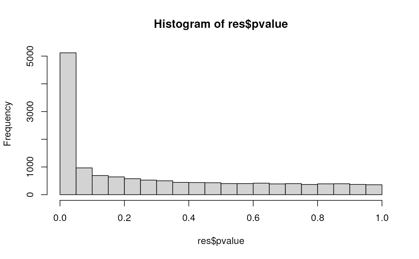
MA-plot and volcano plot
A good way to visualize differential expression is the MA-plot (aka Mean-Difference plot). It consists of a 45-degree rotation of the scatterplot between the treated and control mean expression.
DESeq2::plotMA(res)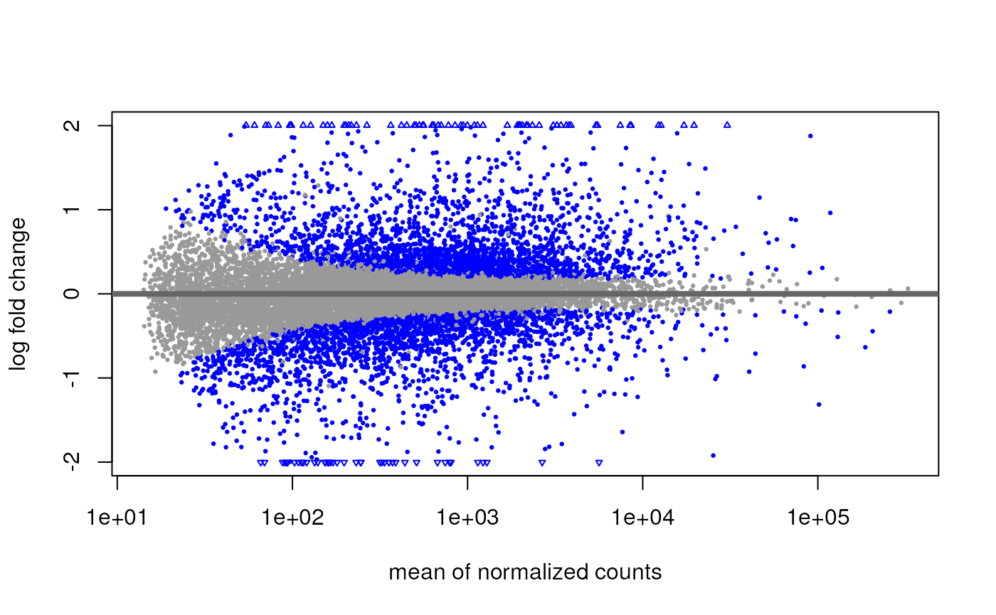
Finally, the volcano plot is a way to simultaneously look at the significance (on the y axis) and effect size (x axis) of differential expression.
ggplot(as.data.frame(res),
       aes(x = log2FoldChange, y = -log10(pvalue), color = padj<=0.05)) +
    geom_point() +
    geom_vline(xintercept = c(-2, 2), linetype = "dotted")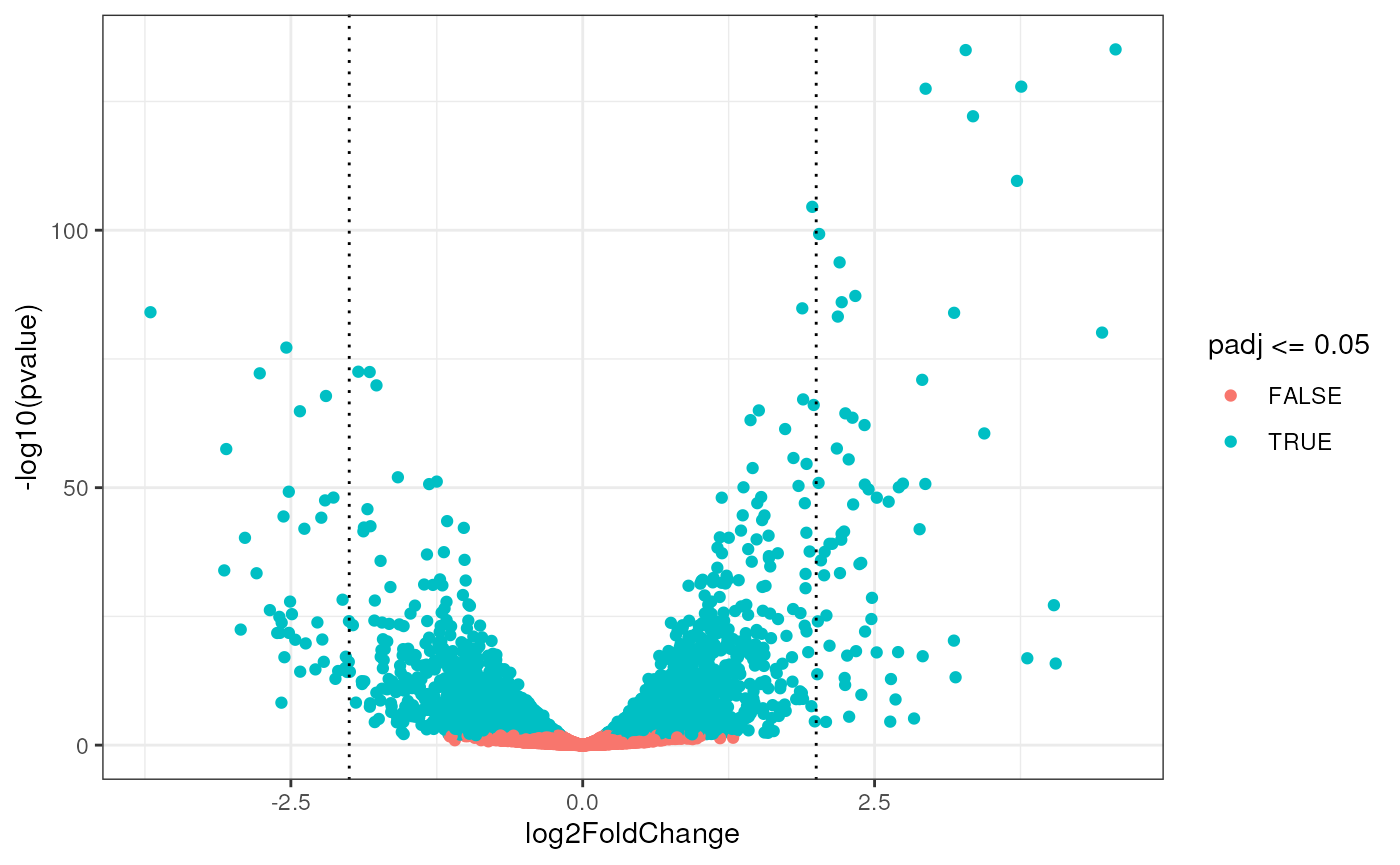
Visualize selected genes
Very often we are interested in looking at the most differentially expressed genes. In this case, we focus on the top 30 genes ordered by p-value and visualize their expression in a heatmap.
vsd <- vst(dds, blind = TRUE)

# Get top DE genes
genes <- res[order(res$pvalue), ] |>
         head(30) |>
         rownames()
heatmapData <- assay(vsd)[genes, ]

# Scale counts for visualization
heatmapData <- t(scale(t(heatmapData)))

# Add annotation
heatmapColAnnot <- data.frame(colData(vsd)[, c("cell", "dex")])
heatmapColAnnot <- HeatmapAnnotation(df = heatmapColAnnot)


# Plot as heatmap
ComplexHeatmap::Heatmap(heatmapData,
                        top_annotation = heatmapColAnnot,
                        cluster_rows = TRUE, cluster_columns = TRUE)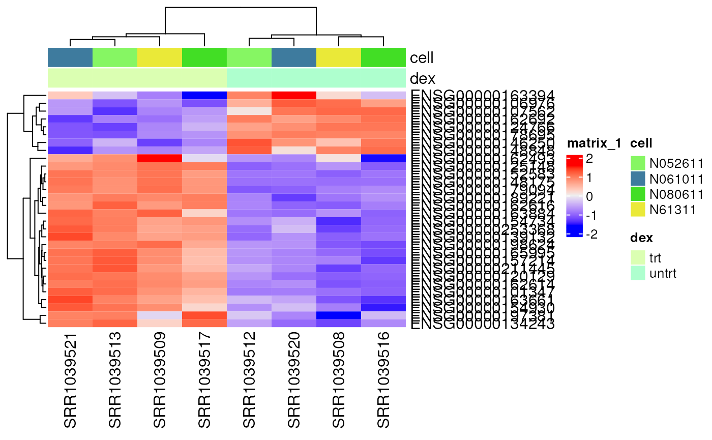
Session Info
## R version 4.3.0 (2023-04-21)
## Platform: x86_64-pc-linux-gnu (64-bit)
## Running under: Ubuntu 22.04.2 LTS
##
## Matrix products: default
## BLAS:   /usr/lib/x86_64-linux-gnu/openblas-pthread/libblas.so.3
## LAPACK: /usr/lib/x86_64-linux-gnu/openblas-pthread/libopenblasp-r0.3.20.so;  LAPACK version 3.10.0
##
## locale:
##  [1] LC_CTYPE=en_US.UTF-8       LC_NUMERIC=C
##  [3] LC_TIME=en_US.UTF-8        LC_COLLATE=en_US.UTF-8
##  [5] LC_MONETARY=en_US.UTF-8    LC_MESSAGES=en_US.UTF-8
##  [7] LC_PAPER=en_US.UTF-8       LC_NAME=C
##  [9] LC_ADDRESS=C               LC_TELEPHONE=C
## [11] LC_MEASUREMENT=en_US.UTF-8 LC_IDENTIFICATION=C
##
## time zone: Etc/UTC
## tzcode source: system (glibc)
##
## attached base packages:
## [1] grid      stats4    stats     graphics  grDevices utils     datasets
## [8] methods   base
##
## other attached packages:
##  [1] ggplot2_3.4.3               ComplexHeatmap_2.16.0
##  [3] edgeR_3.42.4                limma_3.56.2
##  [5] DESeq2_1.40.2               airway_1.20.0
##  [7] SummarizedExperiment_1.30.2 Biobase_2.60.0
##  [9] GenomicRanges_1.52.0        GenomeInfoDb_1.36.2
## [11] IRanges_2.34.1              S4Vectors_0.38.1
## [13] BiocGenerics_0.46.0         MatrixGenerics_1.12.3
## [15] matrixStats_1.0.0
##
## loaded via a namespace (and not attached):
##  [1] tidyselect_1.2.0        farver_2.1.1            dplyr_1.1.2
##  [4] bitops_1.0-7            fastmap_1.1.1           RCurl_1.98-1.12
##  [7] digest_0.6.33           lifecycle_1.0.3         cluster_2.1.4
## [10] magrittr_2.0.3          compiler_4.3.0          rlang_1.1.1
## [13] sass_0.4.7              tools_4.3.0             utf8_1.2.3
## [16] yaml_2.3.7              knitr_1.43              labeling_0.4.2
## [19] S4Arrays_1.0.5          DelayedArray_0.26.7     RColorBrewer_1.1-3
## [22] abind_1.4-5             BiocParallel_1.34.2     withr_2.5.0
## [25] purrr_1.0.2             desc_1.4.2              fansi_1.0.4
## [28] colorspace_2.1-0        scales_1.2.1            iterators_1.0.14
## [31] cli_3.6.1               rmarkdown_2.24          crayon_1.5.2
## [34] ragg_1.2.5              generics_0.1.3          rjson_0.2.21
## [37] cachem_1.0.8            stringr_1.5.0           zlibbioc_1.46.0
## [40] parallel_4.3.0          XVector_0.40.0          vctrs_0.6.3
## [43] Matrix_1.6-1            jsonlite_1.8.7          GetoptLong_1.0.5
## [46] clue_0.3-64             systemfonts_1.0.4       locfit_1.5-9.8
## [49] foreach_1.5.2           jquerylib_0.1.4         glue_1.6.2
## [52] pkgdown_2.0.7           codetools_0.2-19        stringi_1.7.12
## [55] gtable_0.3.4            shape_1.4.6             munsell_0.5.0
## [58] tibble_3.2.1            pillar_1.9.0            htmltools_0.5.6
## [61] GenomeInfoDbData_1.2.10 circlize_0.4.15         R6_2.5.1
## [64] textshaping_0.3.6       doParallel_1.0.17       rprojroot_2.0.3
## [67] evaluate_0.21           lattice_0.21-8          highr_0.10
## [70] png_0.1-8               memoise_2.0.1           bslib_0.5.1
## [73] Rcpp_1.0.11             xfun_0.40               fs_1.6.3
## [76] pkgconfig_2.0.3         GlobalOptions_0.1.2