                   mpg cyl
Mazda RX4         21.0   6
Mazda RX4 Wag     21.0   6
Datsun 710        22.8   4
Hornet 4 Drive    21.4   6
Hornet Sportabout 18.7   8
Valiant 18.1 6Linear models are (almost) all you need to know
Advanced Statistics and Data Analysis
Davide Risso
ANOVA
Analysis of Variance (ANOVA)
Last semester you have seen ANOVA as a generalization of the t-test for more than two groups.
Let’s recall it with an example.
ANOVA example
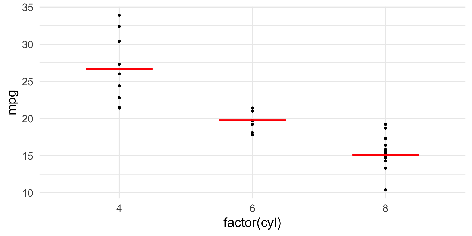
Does car efficiency, measured in miles-per-gallon (mpg), depend on the type of engine?
In our data, we have three engyine types: 4, 6, and 8 cylinder engines.
We can use a one-way ANOVA to test whether the efficiency is the same or different across cars with these engines.
ANOVA example
ANOVA example
ANOVA as a linear model
In fact, we can perform the same analysis as a linear regression, choosing mpg as the response and cyl as a categorical covariate.
For categorical covariates, we need to define dummy variables.
In the case of cyl, which has three levels, we need two dummies (plus the intercept).
Warning
- Why do we need only two dummy variables?
- What would happen if we include all three in the regression?
ANOVA as a linear model
Call:
lm(formula = mpg ~ factor(cyl), data = mtcars)

Residuals:
    Min      1Q  Median      3Q     Max
-5.2636 -1.8357  0.0286  1.3893  7.2364

Coefficients:
             Estimate Std. Error t value Pr(>|t|)
(Intercept)   26.6636     0.9718  27.437  < 2e-16 ***
factor(cyl)6  -6.9208     1.5583  -4.441 0.000119 ***
factor(cyl)8 -11.5636     1.2986  -8.905 8.57e-10 ***
---
Signif. codes:  0 '***' 0.001 '**' 0.01 '*' 0.05 '.' 0.1 ' ' 1

Residual standard error: 3.223 on 29 degrees of freedom
Multiple R-squared:  0.7325,    Adjusted R-squared:  0.714
F-statistic:  39.7 on 2 and 29 DF,  p-value: 4.979e-09
ANOVA as a linear model
As we can see from the F statistic and its p-value, the results are exactly the same.
This is not by coincidence, but because we are performing exactly the same analysis.
In fact, R’s aov function internally calls lm.fit exactly like lm.
The design matrix
To understand mathematically why this is the same thing, we have to introduce the design matrix, which is just another name for the matrix \(X\) whose columns contain the covariates that we include in the model.
When we perform a regression against categorical variables, lm implicitly defines a set of dummy variables to include in the design matrix.
We can see what happens internally, by using the model.matrix function, which transforms the formula we feed into lm into a design matrix.
The design matrix
                  (Intercept) factor(cyl)6 factor(cyl)8
Mazda RX4                   1            1            0
Mazda RX4 Wag               1            1            0
Datsun 710                  1            0            0
Hornet 4 Drive              1            1            0
Hornet Sportabout           1            0            1
Valiant                     1            1            0
Definition
Dummy variables are binary variables that indicate whether each observation belongs to a given category.
Why not all three dummies?
Remember that we need to invert the design matrix \(X\) to obtain the least squares solution: \[ \hat{\beta} = (X^\top X)^{-1} X^\top y. \]
This means that \(X^\top X\) needs to be invertible, which implies that \(X\) is full rank.
Definition
The rank of a matrix is the number of columns that are independent of all the others.
If the rank is equal to the number of columns, the matrix is said to be full rank.
Why not all three dummies?
                    factor(cyl)4 factor(cyl)6 factor(cyl)8
Mazda RX4         1            0            1            0
Mazda RX4 Wag     1            0            1            0
Datsun 710        1            1            0            0
Hornet 4 Drive    1            0            1            0
Hornet Sportabout 1            0            0            1
Valiant 1 0 1 0[1] 3Error in `solve.default()`:
! system is computationally singular: reciprocal condition number = 6.93889e-18ANOVA and linear regression
When we think about ANOVA, we are thinking about comparing the means of three or more groups.
In the mtcars example, we have three groups, and we can think about the following model \[
y_i =
\begin{cases}
\mu_1 + \varepsilon_i & \text{if obs. } i \text{ is in group 1} \\
\mu_2 + \varepsilon_i & \text{if obs. } i \text{ is in group 2} \\
\mu_3 + \varepsilon_i & \text{if obs. } i \text{ is in group 3}
\end{cases}
\]
ANOVA and linear regression
In matrix notation: \[ \begin{bmatrix} y_1 \\ y_2 \\ \vdots \\ y_{i} \\ y_{i+1} \\ \vdots \\ y_{n-1} \\ y_{n} \\ \end{bmatrix} = \begin{bmatrix} 1 & 0 & 0 \\ 1 & 0 & 0 \\ \vdots \\ 0 & 1 & 0 \\ 0 & 1 & 0 \\ \vdots \\ 0 & 0 & 1 \\ 0 & 0 & 1 \\ \end{bmatrix} \begin{bmatrix} \mu_1 \\ \mu_2 \\ \mu_3 \end{bmatrix} + \begin{bmatrix} \varepsilon_1 \\ \varepsilon_2 \\ \vdots \\ \varepsilon_{i} \\ \varepsilon_{i+1} \\ \vdots \\ \varepsilon_{n-1} \\ \varepsilon_{n} \\ \end{bmatrix} \]
ANOVA and linear regression
In linear regression, we define the model as \[ y_i = \beta_0 + \sum_{j=1}^p \beta_j x_{ij} + \varepsilon_i, \]
where \(p\) is the number of covariates in \(X\).
ANOVA and linear regression
In matrix notation: \[ \begin{bmatrix} y_1 \\ y_2 \\ \vdots \\ y_{i} \\ y_{i+1} \\ \vdots \\ y_{n-1} \\ y_{n} \\ \end{bmatrix} = \begin{bmatrix} 1 & 0 & 0 \\ 1 & 0 & 0 \\ \vdots \\ 1 & 1 & 0 \\ 1 & 1 & 0 \\ \vdots \\ 1 & 0 & 1 \\ 1 & 0 & 1 \\ \end{bmatrix} \begin{bmatrix} \beta_0 \\ \beta_1 \\ \beta_2 \end{bmatrix} + \begin{bmatrix} \varepsilon_1 \\ \varepsilon_2 \\ \vdots \\ \varepsilon_{i} \\ \varepsilon_{i+1} \\ \vdots \\ \varepsilon_{n-1} \\ \varepsilon_{n} \\ \end{bmatrix} \]
ANOVA and linear regression
Mathematically, we can see that \[ y = \beta_0 X^{(1)} + \beta_1 X^{(2)} + \beta_2 X^{(3)} + \varepsilon, \] where \(X^{(j)}\) indicates the \(j\)-th column of the design matrix.
Hence, \[ y_i = \begin{cases} \beta_0 + \varepsilon_i &\text{if obs. } i \text{ is in group 1} \\ \beta_0 + \beta_1 + \varepsilon_i & \text{if obs. } i \text{ is in group 2} \\ \beta_0 + \beta_2 + \varepsilon_i & \text{if obs. } i \text{ is in group 3} \end{cases} \]
ANOVA and linear regression
It is now easy to see that:
\(\mu_1 = \beta_0\), i.e., the mean of the reference group;
\(\mu_2 = \beta_0 + \beta_1 \implies \beta_1 = \mu_2 - \mu_1\);
\(\mu_3 = \beta_0 + \beta_2 \implies \beta_2 = \mu_3 - \mu_1\);
This gives an intuitive interpretation of the regression coefficients in the case of dummy variables.
ANOVA and linear regression
We can check this in R.
Contrasts
But what is the average difference between the MPG of 6 and 8 cylinder cars?
Is this difference statistically significant?
To answer this question, we need to compute a linear combination of the parameters, called a contrast.
In fact, \[ \mu_3 - \mu_2 = (\beta_0 + \beta_2) - (\beta_0 + \beta_1) = \beta_2 - \beta_1 \]
We can apply the usual t-test to test the significance of any linear combination of the coefficients.
Contrasts
Advantages of linear modeling
The advantage of the linear model formulation is that we can now include multiple covariates, including continuous ones, and even interactions.
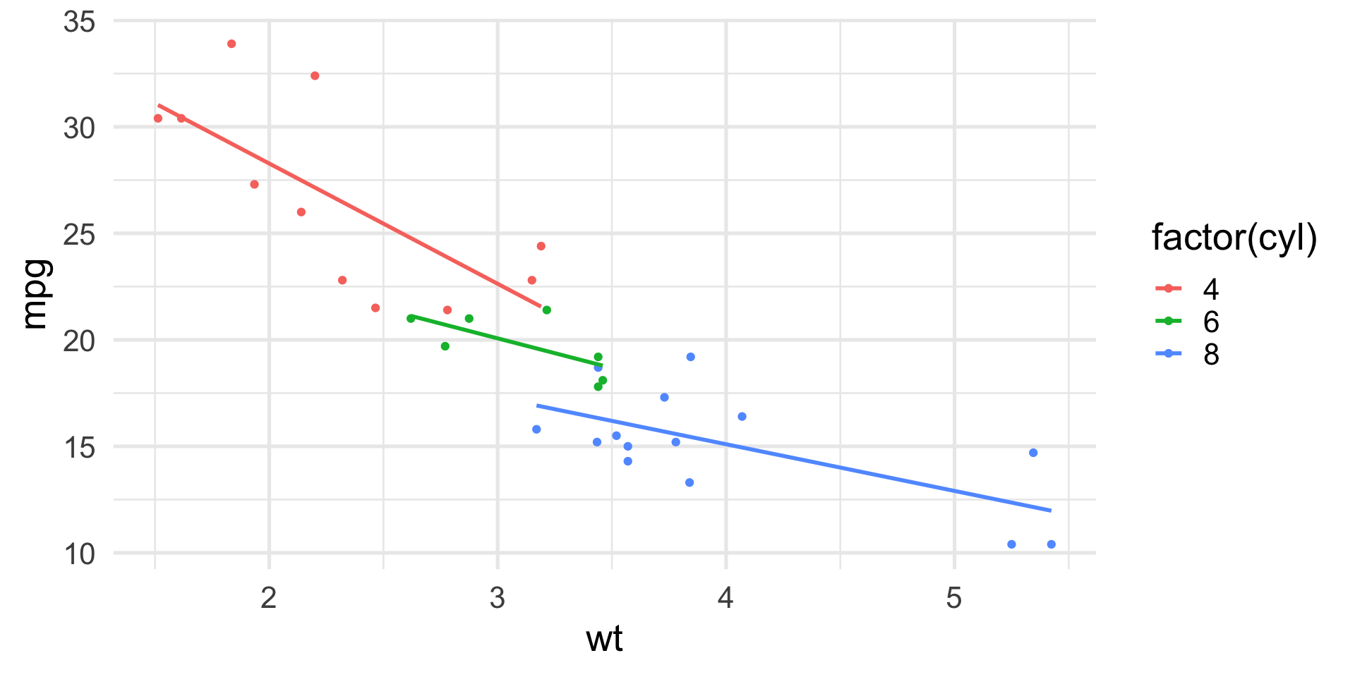
Including weight in the model
If we include weight in the model, we have to include an additional column in the design matrix.
\[ \begin{bmatrix} y_1 \\ y_2 \\ \vdots \\ y_{i} \\ y_{i+1} \\ \vdots \\ y_{n-1} \\ y_{n} \\ \end{bmatrix} = \begin{bmatrix} 1 & 0 & 0 & w_1\\ 1 & 0 & 0 & w_2\\ \vdots \\ 1 & 1 & 0 & w_i\\ 1 & 1 & 0 & w_{i+1}\\ \vdots \\ 1 & 0 & 1 & w_{n-1}\\ 1 & 0 & 1 & w_n\\ \end{bmatrix} \begin{bmatrix} \beta_0 \\ \beta_1 \\ \beta_2 \\ \beta_3 \end{bmatrix} + \begin{bmatrix} \varepsilon_1 \\ \varepsilon_2 \\ \vdots \\ \varepsilon_{i} \\ \varepsilon_{i+1} \\ \vdots \\ \varepsilon_{n-1} \\ \varepsilon_{n} \\ \end{bmatrix} \]
Including weight in the model
Now we have: \[ y_i = \begin{cases} \beta_0 + \beta_3 w_i + \varepsilon_i &\text{if group 1} \\ \beta_0 + \beta_1 + \beta_3 w_i + \varepsilon_i & \text{if group 2} \\ \beta_0 + \beta_2 + \beta_3 w_i + \varepsilon_i & \text{if group 3} \end{cases} \]
This means that the relationship between MPG and weight has the same slope across groups, but start from a different intercept.
Including weight in the model
Call:
lm(formula = mpg ~ factor(cyl) + wt, data = mtcars)

Residuals:
    Min      1Q  Median      3Q     Max
-4.5890 -1.2357 -0.5159  1.3845  5.7915

Coefficients:
             Estimate Std. Error t value Pr(>|t|)
(Intercept)   33.9908     1.8878  18.006  < 2e-16 ***
factor(cyl)6  -4.2556     1.3861  -3.070 0.004718 **
factor(cyl)8  -6.0709     1.6523  -3.674 0.000999 ***
wt            -3.2056     0.7539  -4.252 0.000213 ***
---
Signif. codes:  0 '***' 0.001 '**' 0.01 '*' 0.05 '.' 0.1 ' ' 1

Residual standard error: 2.557 on 28 degrees of freedom
Multiple R-squared:  0.8374,    Adjusted R-squared:   0.82
F-statistic: 48.08 on 3 and 28 DF,  p-value: 3.594e-11
Including interactions
If we include the interactions in the model, we have to include two additional columns in the design matrix, which are obtained by multiplying the two relative columns.
\[ \begin{bmatrix} y_1 \\ y_2 \\ \vdots \\ y_{i} \\ y_{i+1} \\ \vdots \\ y_{n-1} \\ y_{n} \\ \end{bmatrix} = \begin{bmatrix} 1 & 0 & 0 & w_1 & 0 & 0\\ 1 & 0 & 0 & w_2 & 0 & 0\\ \vdots \\ 1 & 1 & 0 & w_i & w_i & 0\\ 1 & 1 & 0 & w_{i+1} & w_{i+1} & 0\\ \vdots \\ 1 & 0 & 1 & w_{n-1} & 0 & w_{n-1} \\ 1 & 0 & 1 & w_n & 0 & w_n\\ \end{bmatrix} \begin{bmatrix} \beta_0 \\ \beta_1 \\ \beta_2 \\ \beta_3 \\ \beta_4 \\ \beta_5 \end{bmatrix} + \begin{bmatrix} \varepsilon_1 \\ \varepsilon_2 \\ \vdots \\ \varepsilon_{i} \\ \varepsilon_{i+1} \\ \vdots \\ \varepsilon_{n-1} \\ \varepsilon_{n} \\ \end{bmatrix} \]
Including interactions
Call:
lm(formula = mpg ~ factor(cyl) * wt, data = mtcars)

Residuals:
    Min      1Q  Median      3Q     Max
-4.1513 -1.3798 -0.6389  1.4938  5.2523

Coefficients:
                Estimate Std. Error t value Pr(>|t|)
(Intercept)       39.571      3.194  12.389 2.06e-12 ***
factor(cyl)6     -11.162      9.355  -1.193 0.243584
factor(cyl)8     -15.703      4.839  -3.245 0.003223 **
wt                -5.647      1.359  -4.154 0.000313 ***
factor(cyl)6:wt    2.867      3.117   0.920 0.366199
factor(cyl)8:wt    3.455      1.627   2.123 0.043440 *
---
Signif. codes:  0 '***' 0.001 '**' 0.01 '*' 0.05 '.' 0.1 ' ' 1

Residual standard error: 2.449 on 26 degrees of freedom
Multiple R-squared:  0.8616,    Adjusted R-squared:  0.8349
F-statistic: 32.36 on 5 and 26 DF,  p-value: 2.258e-10
Including interactions
Now we have: \[ y_i = \begin{cases} \beta_0 + \beta_3 w_i + \varepsilon_i &\text{if group 1} \\ (\beta_0 + \beta_1) + (\beta_3 + \beta_4) w_i + \varepsilon_i & \text{if group 2} \\ (\beta_0 + \beta_2) + (\beta_3 + \beta_5) w_i + \varepsilon_i & \text{if group 3} \end{cases} \]
This means that the relationship between MPG and weight changes both in terms of slope and intercept across groups.
Important
How do you interpret the parameters in this case?
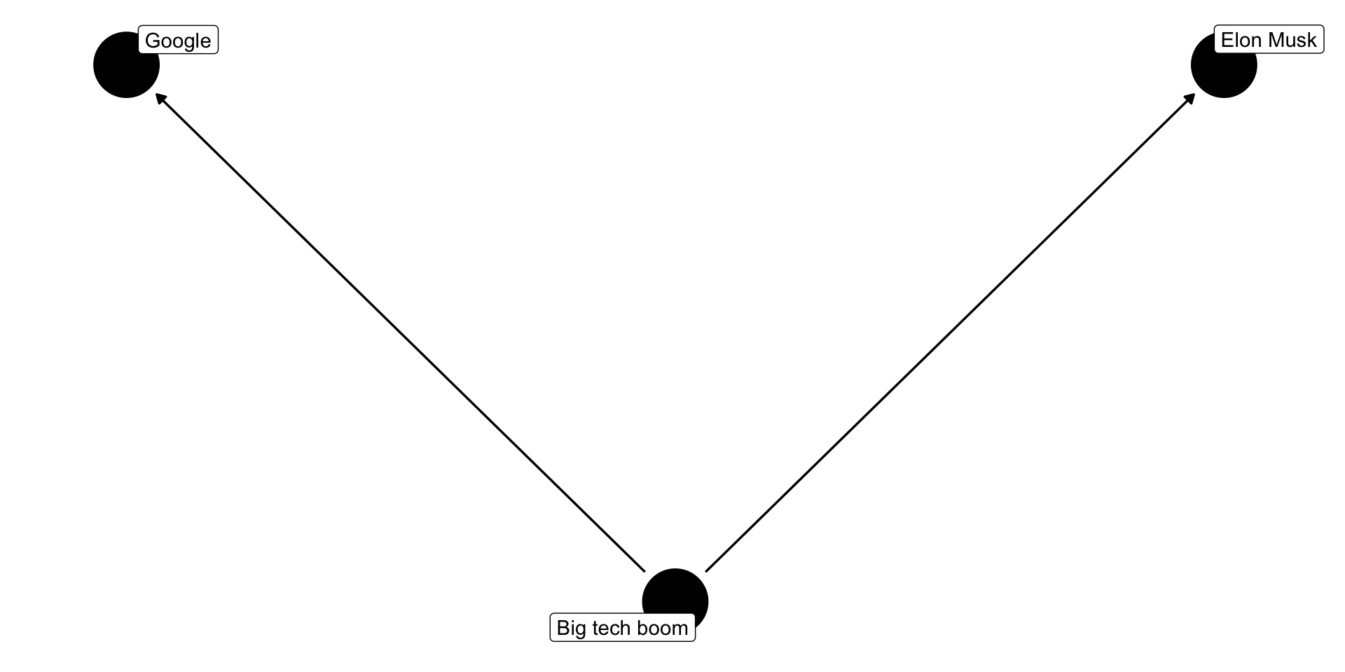
Confounding
Google and Elon Musk
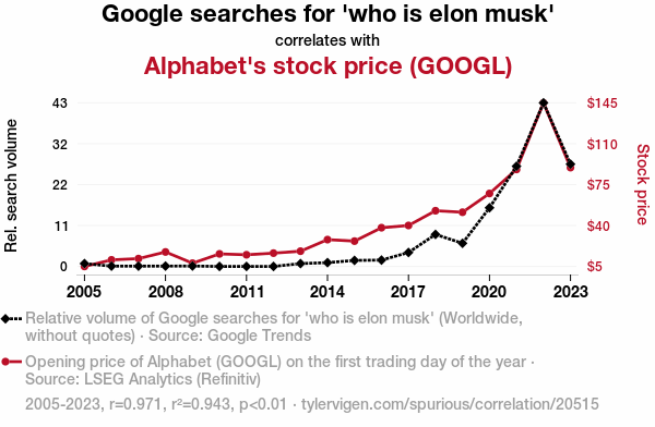
Cause or effect?
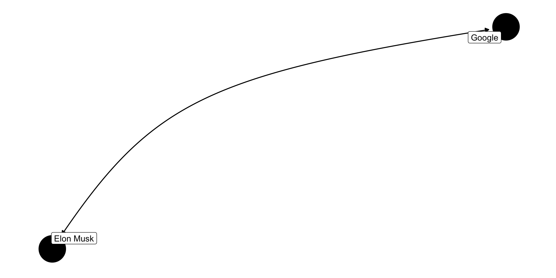
Cause or effect?
Cats vote Democrat!
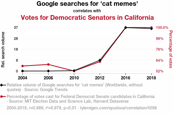
Is this real?
Confounding and spurious correlations
One needs to be careful when interpreting linear models.
Confounding may lead to significant associations that turn out not to be significant or may even be opposite effects!
This is known as the Simpson’s paradox.
Association does not imply causation
A more realistic example
We want to study the fertility rates in Swiss provinces and their relations with some socio-economic indicators.
             Fertility Agriculture Examination Education Catholic
Courtelary        80.2        17.0          15        12     9.96
Delemont          83.1        45.1           6         9    84.84
Franches-Mnt      92.5        39.7           5         5    93.40
Moutier           85.8        36.5          12         7    33.77
Neuveville        76.9        43.5          17        15     5.16
Porrentruy        76.1        35.3           9         7    90.57
             Infant.Mortality
Courtelary               22.2
Delemont                 22.2
Franches-Mnt             20.2
Moutier                  20.3
Neuveville               20.6
Porrentruy               26.6
A more realistic example
Call:
lm(formula = Fertility ~ Agriculture, data = swiss)

Residuals:
     Min       1Q   Median       3Q      Max
-25.5374  -7.8685  -0.6362   9.0464  24.4858

Coefficients:
            Estimate Std. Error t value Pr(>|t|)
(Intercept) 60.30438    4.25126  14.185   <2e-16 ***
Agriculture  0.19420    0.07671   2.532   0.0149 *
---
Signif. codes:  0 '***' 0.001 '**' 0.01 '*' 0.05 '.' 0.1 ' ' 1

Residual standard error: 11.82 on 45 degrees of freedom
Multiple R-squared:  0.1247,    Adjusted R-squared:  0.1052
F-statistic: 6.409 on 1 and 45 DF,  p-value: 0.01492
A more realistic example
Call:
lm(formula = Fertility ~ Agriculture + Education + Catholic,
data = swiss)
Residuals:
Min 1Q Median 3Q Max
-15.178 -6.548 1.379 5.822 14.840
Coefficients:
Estimate Std. Error t value Pr(>|t|)
(Intercept) 86.22502 4.73472 18.211 < 2e-16 ***
Agriculture -0.20304 0.07115 -2.854 0.00662 **
Education -1.07215 0.15580 -6.881 1.91e-08 ***
Catholic 0.14520 0.03015 4.817 1.84e-05 ***
---
Signif. codes: 0 '***' 0.001 '**' 0.01 '*' 0.05 '.' 0.1 ' ' 1
Residual standard error: 7.728 on 43 degrees of freedom
Multiple R-squared: 0.6423, Adjusted R-squared: 0.6173
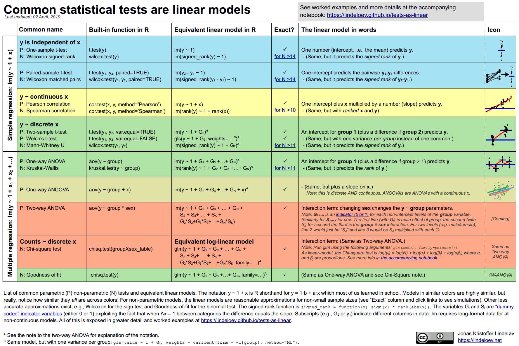
F-statistic: 25.73 on 3 and 43 DF, p-value: 1.089e-09(Almost) everything is a linear model!
The flexibility of linear models
As nicely shown by Jonas Kristoffer Lindelov in his blog post, common statistical tests are linear models:
Example: t-test
Assume that we have measured gene ESR1 in a cohort of patients with breast cancer and we want to test if its expression is the same or different between patients with grade 1 or grade 3 tumors.
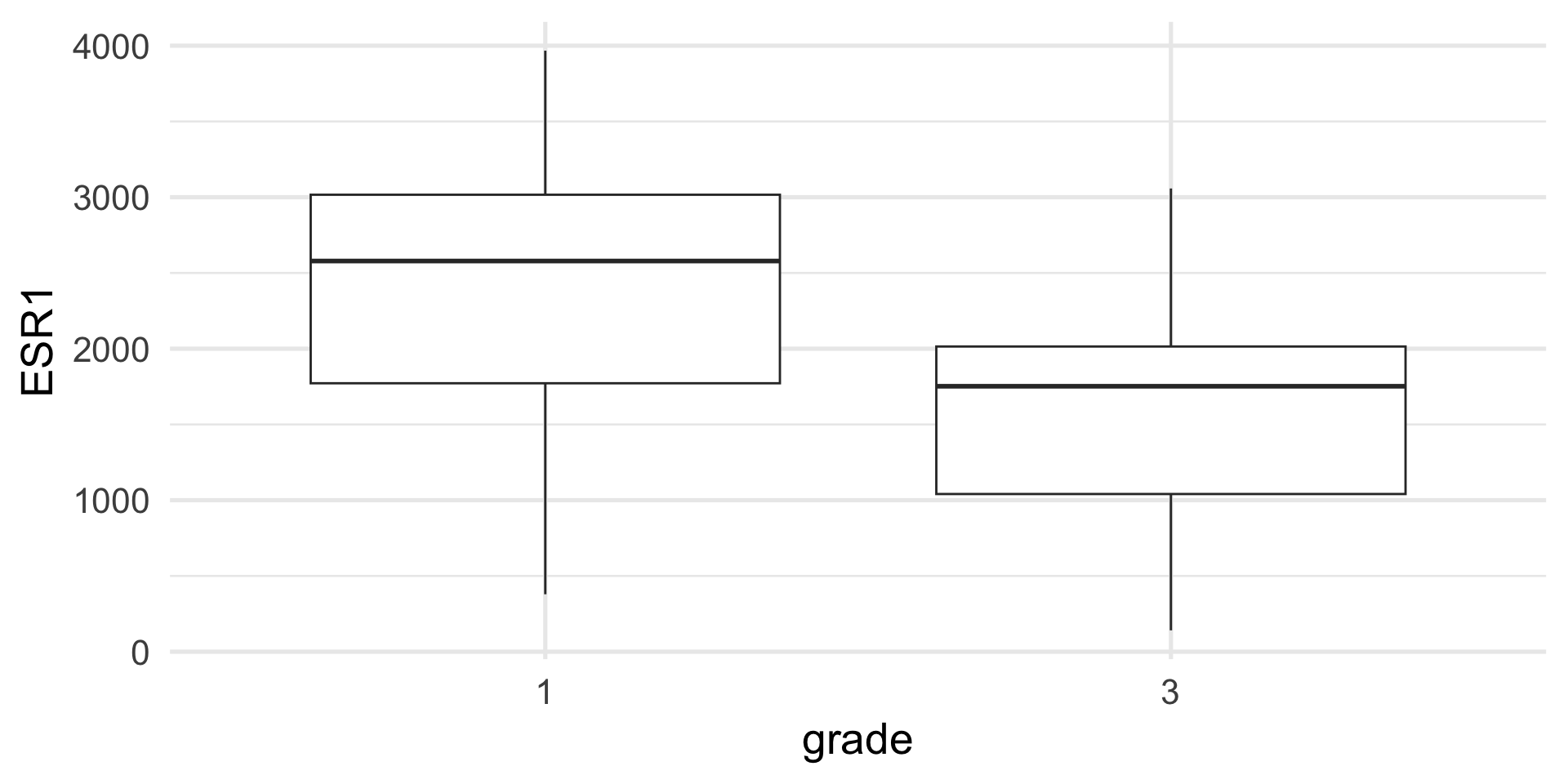
Example: t-test
Assuming that the data are normal, we can use a t-test.
    Two Sample t-test

data:  ESR1 by grade
t = 2.013, df = 30, p-value = 0.05316
alternative hypothesis: true difference in means between group 1 and group 3 is not equal to 0
95 percent confidence interval:
  -10.45303 1448.48516
sample estimates:
mean in group 1 mean in group 3
       2349.383        1630.367
Example: t-test
An equivalent way to perform this test is by fitting a linear model, using the gene expression as response variable and grade as a categorical (binary) covariate.
Call:
lm(formula = ESR1 ~ grade, data = brca)

Residuals:
    Min      1Q  Median      3Q     Max
-1970.2  -589.6   195.4   572.7  1617.8

Coefficients:
            Estimate Std. Error t value Pr(>|t|)
(Intercept)   2349.4      252.6   9.302  2.4e-10 ***
grade3        -719.0      357.2  -2.013   0.0532 .
---
Signif. codes:  0 '***' 0.001 '**' 0.01 '*' 0.05 '.' 0.1 ' ' 1

Residual standard error: 1010 on 30 degrees of freedom
Multiple R-squared:  0.119, Adjusted R-squared:  0.08963
F-statistic: 4.052 on 1 and 30 DF,  p-value: 0.05316