     x1 x2
[1,]  1  7
[2,]  4  7
[3,] 6 2 [,1] [,2]
[1,] 1 7
[2,] 4 7
[3,] 6 2Advanced Statistics and Data Analysis
Linear algebra, also called matrix algebra, and its mathematical notation greatly facilitates the understanding of the concepts behind linear models.
Here, we spend some time to review key concepts of linear algebra, with particular focus on matrix operations and matrix notation.
We will also see how to perform matrix operations in R.
Linear algebra was created to solve systems of linear equations, e.g.
\[\begin{align*} a + b + c &= 6\\ 3a - 2b + x &= 2\\ 2a + b - c &=1 \end{align*}\]
which becomes, in matrix notation,
\[ \begin{bmatrix} 1 & 1 & 1 \\ 3 & -2 & 1 \\ 2 & 1 & -1 \end{bmatrix} \begin{bmatrix} a \\ b \\ c \end{bmatrix} = \begin{bmatrix} 6 \\ 2 \\ 1 \end{bmatrix} \]
The system is solved by
\[ \begin{bmatrix} a \\ b \\ c \end{bmatrix} = \begin{bmatrix} 1 & 1 & 1 \\ 3 & -2 & 1 \\ 2 & 1 & -1 \end{bmatrix}^{-1} \begin{bmatrix} 6 \\ 2 \\ 1 \end{bmatrix} \]
where the \(-1\) denotes the inverse of the matrix.
We can borrow this notation to solve linear models in statistics.
We define vectors as column vectors, i.e., matrices with just one column.
This means that all the operations defined for matrices will be applicable to vectors as well.
We can write matrices by either concatenating vectors or by explicitly writing their elements.
\[ Y = \begin{bmatrix} Y_1 \\ Y_2 \\ \vdots \\ Y_n \end{bmatrix} \quad \quad X = [X_1 \, X_2] = \begin{bmatrix} X_{1,1} & X_{1, 2}\\ X_{2,1} & X_{2, 2}\\ \vdots & \vdots\\ X_{n,1} & X_{n,2} \end{bmatrix} \]
We already know how to create these objects in R
Here, we review some of the operations that can be performed on matrices, both in mathematical terms and in R.
This is the simplest operation: each element of the matrix is multiplied by the scalar.
R automatically recognize a scalar and a matrix and “does the right thing.”
Transposition is a simple operation that simply changes columns to rows. We use \(\top\) sign to denote the transposed of a matrix.
\[ X^\top = \begin{bmatrix} X_{1,1} & \ldots & X_{n, 1}\\ X_{1,2} & \ldots &X_{n, 2}\\ \vdots & \ddots &\vdots\\ X_{1,p} & \ldots & X_{n,p} \end{bmatrix} \]
In R, we can use the t() operator to transpose a matrix.
If \(A\) is an \(n \times m\) matrix and \(B\) is an \(m \times p\) matrix, their matrix product \(X = AB\) is an \(n \times p\) matrix, in which each row of \(A\) is multiplied by each column of \(B\) and summed.
In R, we can use the %*% operator.
In general, the matrix multiplication operator is
For scalars we have the number \(1\), a number such that \(1 x = x\) for any \(x\).
The analogous for matrices, is the identity matrix \[ I = \begin{bmatrix} 1 & 0 & 0 & \ldots & 0 & 0\\ 0 & 1 & 0 & \ldots & 0 & 0\\ 0 & 0 & 1 & \ldots & 0 & 0\\ \vdots & \vdots & \vdots & \ddots & \vdots & \vdots\\ 0 & 0 & 0 & \ldots & 1 & 0\\ 0 & 0 & 0 & \ldots & 0 & 1 \end{bmatrix} \]
By definition, for any matrix \(X\), \(X \, I = X\).
In R we can use the function diag().
     [,1] [,2]
[1,]    1    7
[2,]    4    7
[3,] 6 2 [,1] [,2]
[1,] 1 7
[2,] 4 7
[3,] 6 2Warning
Note the different behavior of diag(x) when x is a scalar or a vector!
A matrix is called square if it has the same number of rows and columns.
The inverse of a square matrix \(X\), denoted by \(X^{-1}\) is the matrix that when multiplied by \(X\) returns the identity matrix.
\[ X \, X^{-1} = I. \]
Note that not all matrices have a defined inverse.
We will see later how this plays a role for linear models.
If the inverse exists, it can be computed using solve().
     [,1] [,2]
[1,]    5    7
[2,] 6 2 [,1] [,2]
[1,] -0.0625 0.21875
[2,] 0.1875 -0.15625 [,1] [,2]
[1,] 1 2.220446e-16
[2,] 0 1.000000e+00Warning
The solve() function is numerically unstable and should be used with caution.
Why do we need linear algebra and matrix notation in statistics?
Linear algebra is a very convenient and compact mathematical way of formalizing many of the concepts of statistics, especially with regards to linear models.
Let’s focus on a couple of simple examples.
Assume that we have a vector \(X\) that contains the data for a sample of \(n\) observations. We can use matrix notation to denote the sample mean of that vector.
Define a \(n \times 1\) matrix \(\mathbf{1} = [1 \, \ldots \, 1]^\top\).
We can compute the mean simply as \(\frac{1}{n} \mathbf{1}^\top X\). \[ \frac{1}{n} \mathbf{1}^\top X = \frac{1}{n} [1 \, \ldots \, 1] \begin{bmatrix} X_1\\ \vdots\\ X_n \end{bmatrix} = \frac{1}{n} \sum_{i=1}^n X_i = \bar{X}. \]
The same is true for the variance: We can simply multiply the centered matrix by its transpose to compute it.
\[ R = X - \bar{X} = \begin{bmatrix} X_1 - \bar{X}\\ \vdots\\ X_n - \bar{X} \end{bmatrix} \]
Then, \[ \frac{1}{n-1} R^\top R = \frac{1}{n-1} \sum_{i=1}^n (X_i - \bar{X})^2. \]
crossprod functionThe operation \(X^\top Y\) is so important in statistics that R has a shortcut function for it, the crossprod() function.
crossprod functionThe crossprod function can be used to compute the variance.
Note that crossprod(r) is a further shortcut for crossprod(r, r).
If we want to measure the linear association between two continuous variables, we can use the correlation coefficient.
An alternative way to look at the association between two variables is to determine the best line that describe their relationship.
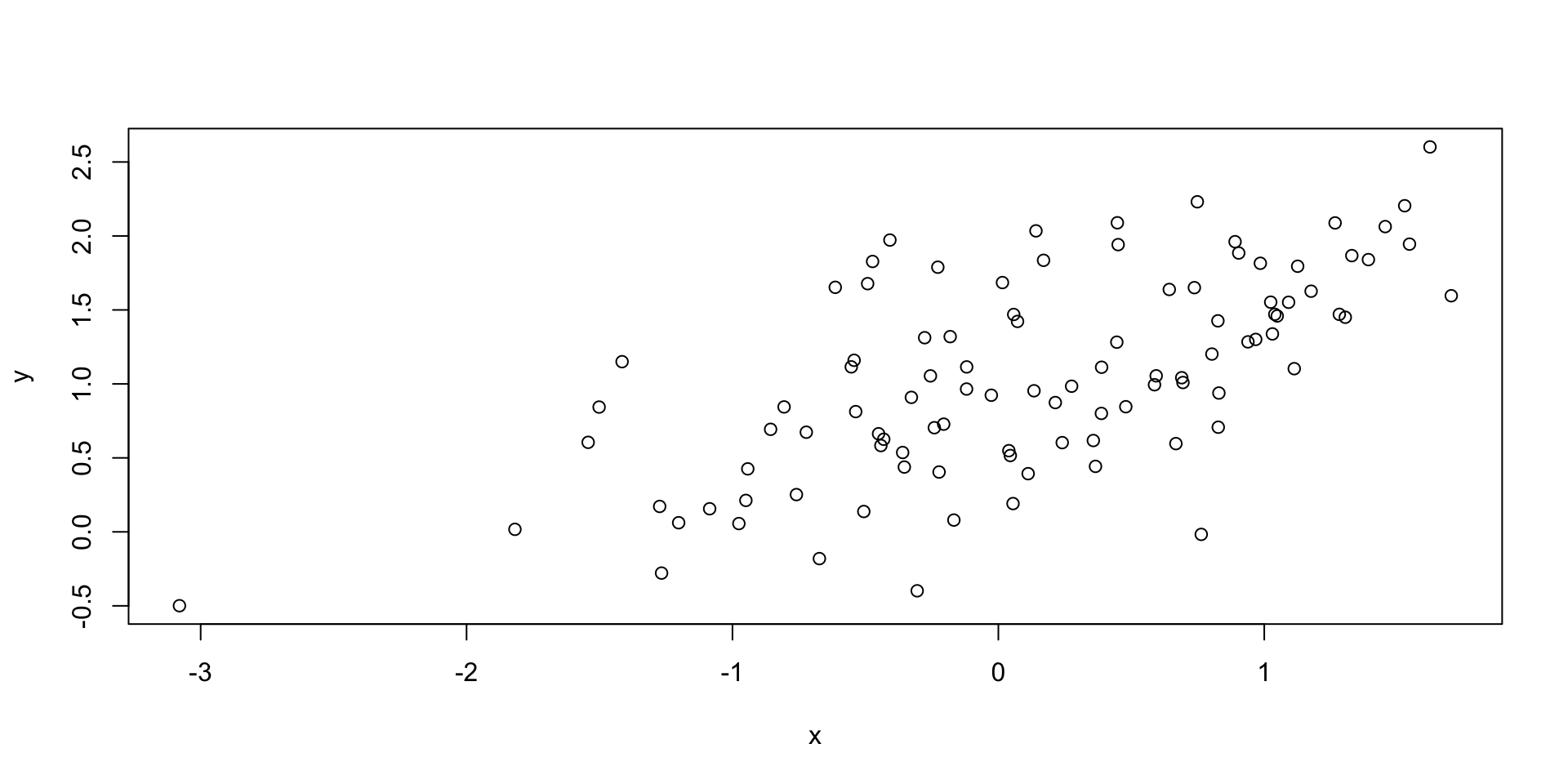
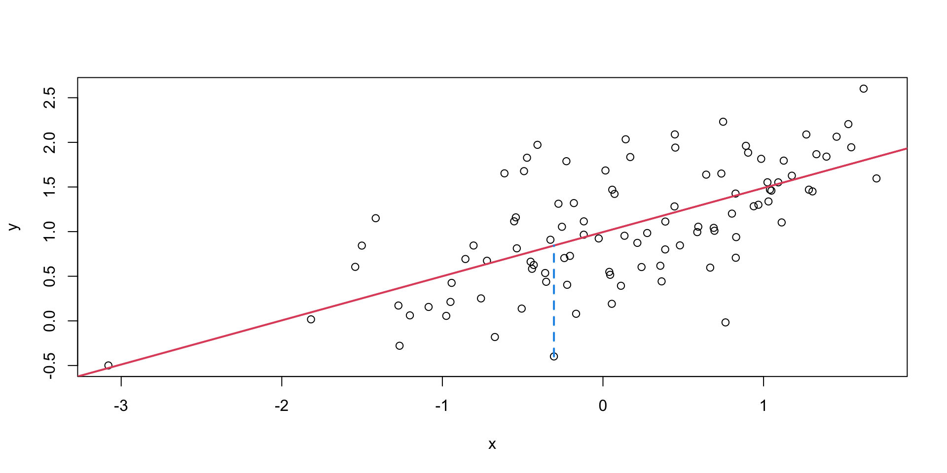
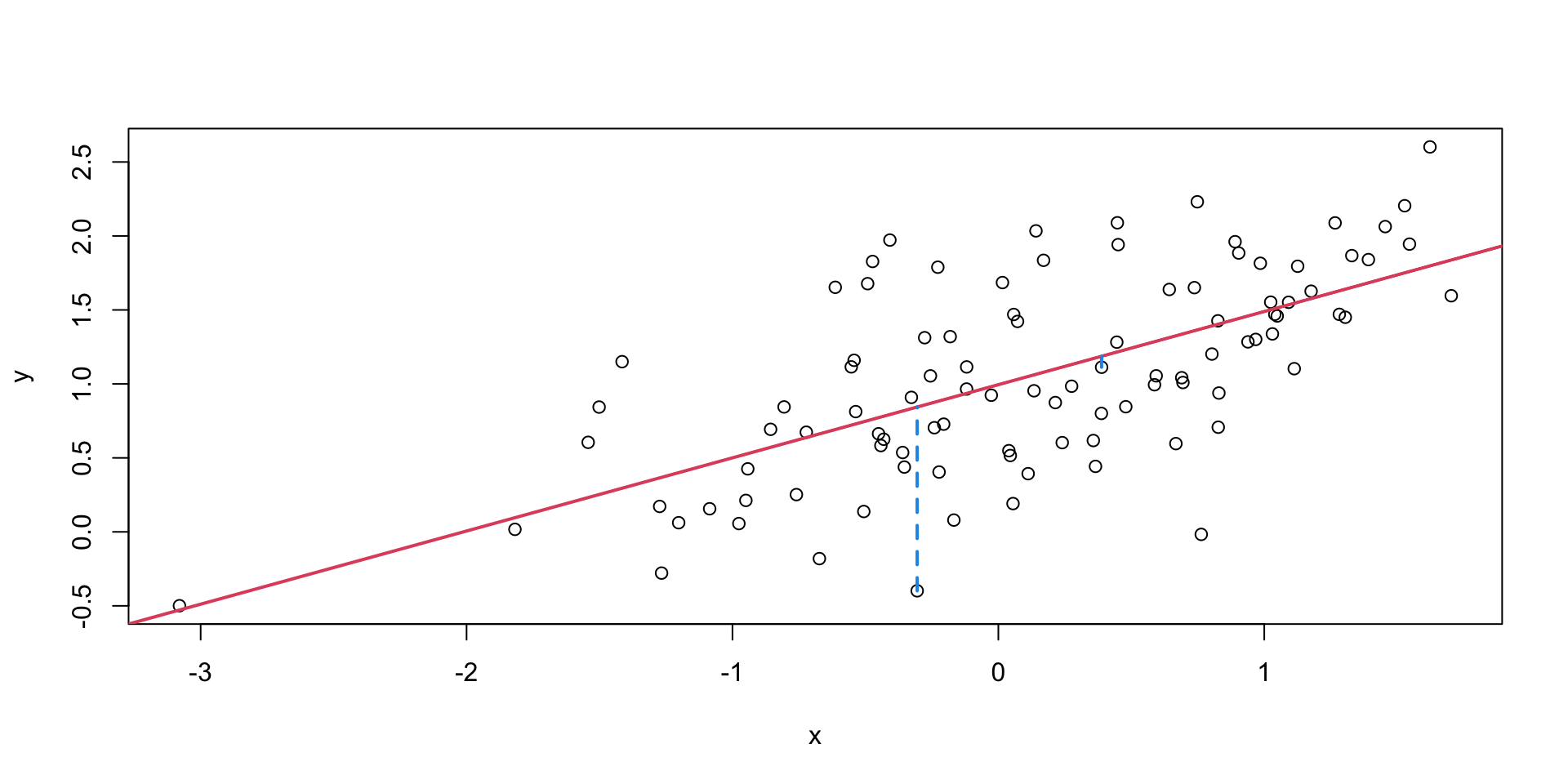
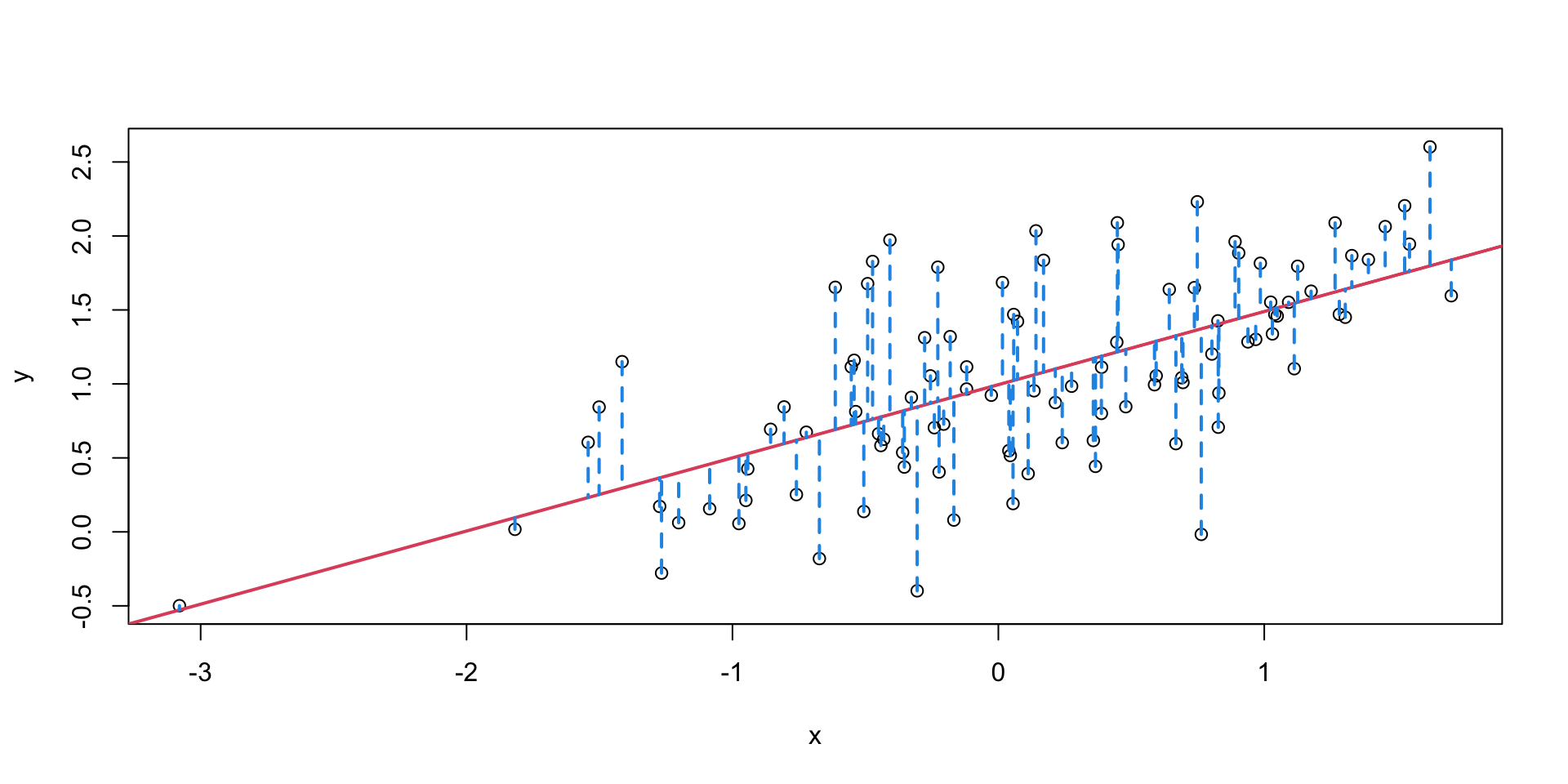
What do we mean by “best”? In the context of regression, “best” means the line that minimizes the sum of squared distances.
Mathematically, we can describe the linear relation between the two quantities \(x\) and \(y\) as \[ \hat{y} = \alpha + \beta x. \]
Finding the best line corresponds to minimize the sum of squared distances between the values of \(y\) and the values of \(\alpha + \beta x\), i.e. \[ \min_{\alpha, \beta} \sum_{i=1}^n (y_i - (\alpha + \beta x_i))^2. \]
To minimize this quantity, as usual, we compute the partial derivatives.
\[\begin{align*} \frac{\partial}{\partial \alpha} &= -2 \sum_{i=1}^n (y_i - \alpha - \beta x_i) = 0,\\ \frac{\partial}{\partial \beta} &= -2 \sum_{i=1}^n (y_i - \alpha - \beta x_i) (x_i) = 0,\\ \end{align*}\]
We can show that \[\begin{align*} \alpha &= \bar{y} - \beta \bar{x},\\ \beta &= \frac{\sum_{i=1}^n (x_i - \bar{x})(y_i - \bar{y})}{\sum_{i=1}^n (x_i - \bar{x})^2} = \frac{\text{Cov}(x, y)}{\text{Var}(x)}. \end{align*}\]
The ideas of linear regression can be applied in the case where we have more than one covariate.
Instead of fitting the line \(\hat{y} = \alpha + \beta x\), we can consider the more general form \[ \hat{y} = \alpha + \beta_1 x_1 + \ldots + \beta_p x_p, \] where \(p\) is the number of covariates and \(x_1, \ldots, x_p\) are \(p\) variables.
For symmetry, the intercept \(\alpha\) is often denoted with \(\beta_0\).
Given a set of \(n\) independent observations, and \(p\) covariates, with \(n > p\), the linear regression model is defined, in matrix notation, as \[ \hat Y = X \beta, \] where
The least-square equation is easier in matrix notation:
\[ (Y - X\beta)^\top (Y - X\beta) \]
The derivative in matrix notation is \[ 2 X^\top (Y - X\beta) = 0 \] which leads to \[ X^\top X \beta = X^\top Y \] and \[ \hat\beta = (X^\top X)^{-1}X^\top Y \]
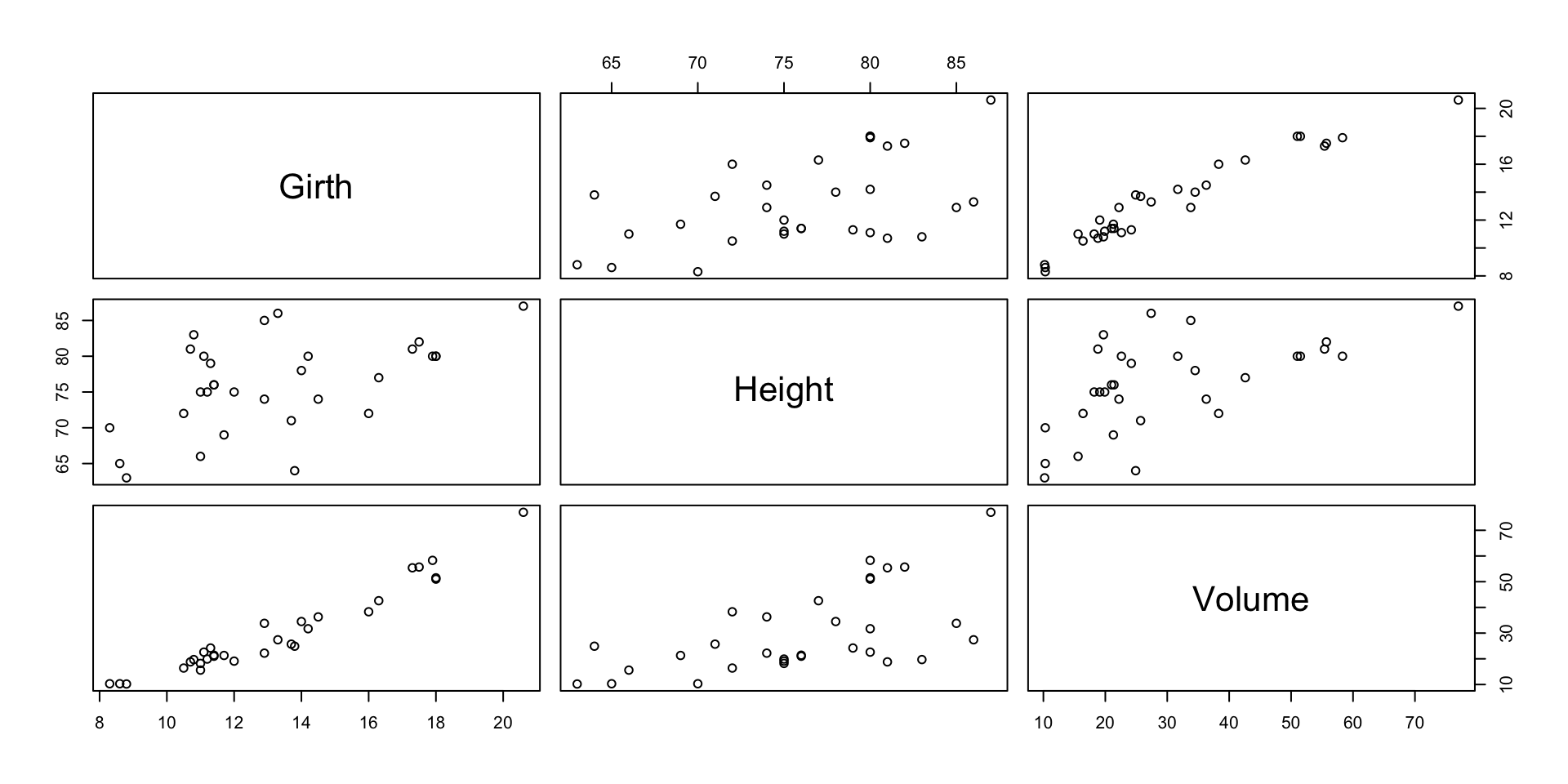
For the Cherry tree data, assume to model the volume (\(y\)) of the trees as a function of girth (\(x_1\)) and height (\(x_2\)): \[ Y_i=\beta_0+ \beta_1 x_{i1}+ \beta_2 x_{i2}+\varepsilon_i\,,\,\,\, i=1, \ldots, 31. \]
This yields
Up until now, we have only defined the regression line as a mathematical entity that we can compute starting from a vector \(y\) and a matrix \(X\).
However, in inferential statistics, both \(Y\) and \(X\) are random variables, and what we observe are the values of our random sample from the population.
This means that what we want to infer the true relationship between \(X\) and \(Y\) in the population starting from the relationship that we observe in the sample.
In other words, there is a true parameter \(\beta\) in the population, and we need to estimate it with the values of our sample.
In the context of inference, regression is often referred to as the linear model.
Suppose that, on \(n\) cases, we observe a continuous response \(y_i\) and one explanatory variable \(x_{i}\).
A simple linear model postulates that the observations are realizations of independent rv’s \(Y_i\) such that: \[ E(Y_i | X_i = x_i)= \beta_0 + \beta_1 x_{i}, \,\,\,i=1,\,\,\,\ldots,n. \]
Therefore, observations are realizations of independent rv’s whose averages lie on the straight line \(\beta_0 + \beta_1 x\).
Another way to look at this is: \[ Y_i = \beta_0 + \beta_1 x_{i} + \varepsilon_i\,\,\,i=1,\ldots,n, \] where \(\varepsilon_i\) are random errors with mean 0.
Often, it is assumed that the variance of the error terms, for all \(i=1,\ldots,n\), is the same, i.e., errors are homoschedastic.
Consider two subjects:
The expected difference in the response of the two subjects is: \[ E(Y_B) - E(Y_A) = \beta_0 + \beta_1 (x_{A}+1) - \beta_0 - \beta_1 x_{A}=\beta_1, \] i.e., \(\beta_1\) is the effect of a one unit increase in \(x.\)
In multiple linear regression, rather than one predictor, we have more than one, \(p\), say. \[ Y_i = \beta_0 + \beta_1 x_{i1} + \ldots +\beta_p x_{ip} + \varepsilon_i\,\,\,i=1,\ldots,n \]
or equivalently \[Y = X\beta + \varepsilon.\]
Consider two subjects:
Expected difference in the response of the two subjects: \[ \begin{aligned} E(Y_B) - E(Y_A) &=&\beta_0 + \beta_1 x_{A1} + \beta_2 (x_{A2}+1)+ \ldots + \beta_p x_{Ap}+\\ && - \beta_0 - \beta_1 x_{A1} - \beta_2 x_{A2}- \ldots - \beta_p x_{Ap}\\ &=&\beta_2,\end{aligned} \] i.e., \(\beta_2\) is the effect of a one unit increase in \(x_2\) for fixed level of the other predictors.
Coefficients \(\beta_1, \ldots, \beta_p\) are called (partial) regression coefficients because they “allow” for the (partial) effect of other variables.
Given a set of \(n\) independent observations, and \(p\) covariates, with \(n > p\), the linear model is defined, in matrix notation, as \[ Y = X \beta + \varepsilon, \] where
As with all the statistical models, it is always a good idea to identify the observed / unobserved quantities, as well as the random / fixed quantities.
In this case,
In some books, \(X\) is not considered a random variable, but a fixed quantity. In this course, we will consider it random, but we will condition our analysis to the observed values of \(X\).
For practical purposes, we do not care about the random variation of \(X\).
The term linear in the linear model refers to the linearity of the model with respect to the parameter \(\beta\).
It does not imply that we have linearity in \(X\) and \(X\) may contain non-linear transformation of the data. For instance the following models are valid linear models.
\[ Y = \beta_0 + \beta_1 X + \beta_2 X^2 + \varepsilon \]
\[ Y = \beta_0 + \beta_1 \log X + \varepsilon \]
Recall that \[ \hat\beta = (X^\top X)^{-1}X^\top Y. \]
This means that \(X^\top X\) needs to be invertible, which implies that \(X\) is full rank.
Definition
The rank of a matrix is the number of columns that are independent of all the others.
If the rank is equal to the number of columns, the matrix is said to be full rank.
This is often referred to as the non collinearity condition.
As with all the statistical models, we need some assumptions.
As a consequence of these assumptions, we can see that the conditional expectation of \(Y\) is
\[ E[Y | X] = X\beta. \]
Exercise
Why?
Explanation
Here the idea is the that system under study really is (approximately) linear, and we are interested in the coefficients per se.
It is often of particular interest to find a minimal set of explanatory variables.
Example
We can use a linear model to understand the effect of a certain treatment on gene expression.
We want to understand which genes are affected by the treatment and why.
Prediction
Here a model is a convenient means to create predictions for new cases.
The only interest is in the quality of the predictions.
Example
We can use a linear model to predict whether a patient will react to a therapy based on their gene expression
We want to get the best possible prediction, we do not care much about which genes are involved.
Fitting the model: how do we estimate \((\beta, \sigma^2)\)?
Inference: what can we say about \(\beta\) (rarely, about \(\sigma^2\)) based on the \(n\) observations?
We do not observe the true parameter \(\beta\) and we need to estimate it from the data.
Luckily, we already know how to estimate \(\beta\), as the value that minimizes the sum of the squares of the differences between \(Y\) and \(X\beta\).
The value of \(\beta\) such that \[ \hat\beta=(X^\top X)^{-1}X^\top y. \] is called the ordinary least squares (OLS) estimator.
To estimate the variance of the random terms, it seems natural to consider the variability of the residuals. An unbiased estimator for \(\sigma^2\) is given by \[ s^2=\displaystyle\frac{\sum(y_i - \hat y_i)^2}{n-p}. \]
In matrix form we have that: \[ \hat y = X\hat\beta, \]
\[ e=y - \hat y, \]
\[ s^2=e^\top e/(n-p)=(y - \hat y)^\top(y - \hat y)/(n-p). \]
We can prove that \(\hat\beta\) is conditionally unbiased, i.e., \[ E[\hat \beta | X] = \beta. \]
The variance of the OLS estimator is
\[ Var(\hat\beta | X) = \sigma^2 (X^\top X)^{-1}. \]
\[\begin{align*} \hat\beta &= (X^\top X)^{-1} X^\top (X\beta + \varepsilon)\\ &= (X^\top X)^{-1} X^\top X\beta + (X^\top X)^{-1} X^\top \varepsilon\\ &= \beta + (X^\top X)^{-1} X^\top \varepsilon. \end{align*}\]
Hence, \[ \hat\beta = \beta + \eta \quad \text{where} \quad \eta = (X^\top X)^{-1} X^\top \varepsilon. \]
To show that \(E[\hat \beta | X] = \beta\), we need to show that \(E[\eta | X] = 0.\)
\[ E[\eta | X] = (X^\top X)^{-1} X^\top E[\varepsilon | X]. \]
Since \(\varepsilon {\perp\!\!\!\!\perp} X\), conditioning on \(X\) does not influence the distribution of \(\varepsilon\), and we know by assumption that \(E[\varepsilon] = 0\). Hence, \[ E[\hat\beta | X] = \beta. \]
As it is true in general for estimation, it is not enough to have a point estimate of the regression parameter, but we want to know what is the distribution of the estimator.
First, we need to compute the standard errors of \(\hat\beta\).
In order to do that we have to remember the assumptions of the linear model, especially those related to the error term \(\varepsilon\).
We denote with \(\Sigma\) the variance/covariance matrix of the error term. In particular, \[ \Sigma_{i,j} = Cov(\varepsilon_i, \varepsilon_j) = \begin{cases} \sigma^2 & i=j\\ 0 & i \neq j \end{cases} \]
Hence, we can write \[ \Sigma = \sigma^2 I. \]
As a consequence, the conditional variance of \(Y\) is \[ Var(Y | X) = Var(X\beta + \epsilon| X) = Var(\epsilon) = \sigma^2 I \]
In matrix notation, the variance of a linear combination \(AY\) can be computed as \[ Var(AY) = A Var(Y) A^\top \]
Since \(\hat\beta\) is a linear combination of \(Y\), we can use the same rule to compute its variance.
\[\begin{align*} Var(\hat\beta | X) &= Var((X^\top X)^{-1} X^\top Y | X)\\ &= (X^\top X)^{-1} X^\top Var(Y | X) ((X^\top X)^{-1} X^\top)^\top. \end{align*}\]
Note that:
Hence, \[ ((X^\top X)^{-1} X^\top)^\top = X (X^\top X)^{-1} \]
Therefore,
\[\begin{align*} Var(\hat\beta | X) &= (X^\top X)^{-1} X^\top Var(Y|X) X (X^\top X)^{-1} \\ &= (X^\top X)^{-1} X^\top \sigma^2 I X (X^\top X)^{-1}\\ &= \sigma^2 (X^\top X)^{-1} X^\top X (X^\top X)^{-1}\\ &= \sigma^2 (X^\top X)^{-1}. \end{align*}\]
Hence, the diagonal of the square root of this matrix contains the standard errors of \(\beta\).
If we could observe \(\varepsilon\), we could simply estimate \(\sigma^2\) by \[ \hat\sigma^2 = \frac{1}{n} \sum_{i=1}^n \varepsilon_i^2. \]
Since we do not observe \(\varepsilon\), we can use the residuals \(e = Y - X\hat\beta\).
We also need to correct for the degrees of freedom (more on this later), to get our estimator: \[ s^2 = \frac{1}{n-p} \sum_{i=1}^n e_i^2. \]
This estimator is conditionally unbiased, i.e., \[ E[s^2 | X] = \sigma^2. \]
The fact that we divide by \(n-p\) derives from the proof that \(\hat\sigma^2\) is unbiased.
This proof is quite complicated mathematically, so we will skip it for now.
However, it derives from the geometric interpretation of regression, which we will see if we have time at the end of the course.
For now, notice that because we assumed that \(n > p\), we do not have problems in estimating \(\sigma^2\).
Also, note the similarity with the usual estimator of the variance: Here, instead of \(n - 1\) we use \(n-p\), because we have \(p\) parameters, and hence \(n-p\) degrees of freedom.
Note which assumptions we did not need to get to these results.
These results ensure that linear models can be applied in a lot of different settings, without requiring too stringent assumptions.
Remember that for now, we did not make any assumptions about the distribution of the data. We only assumed that:
For the next results to hold, we need to restrict our model to the following assumption: \[ \varepsilon_i \overset{iid}{\sim} N(0, \sigma^2). \]
We need the normality assumption in order to make inference on the coefficients of the model, i.e., to create confidence intervals and test hypotheses on the parameter \(\beta\).
The main results that we will see are the \(t\)-test and the \(F\)-test.
It can be proved that:
\(\hat\beta \sim N_p(\beta, \sigma^2(X^\top X)^{-1})\);
\((n-p)s^2/\sigma^2 \sim \chi^2_{n-p}\);
\(\hat\beta\) and \(s^2\) are independent rv.
We have, for \(j=1,\ldots,p\)
\(\hat\beta_j\sim N(\beta_j, \sigma^2[(X^\top X)^{-1}]_{jj})\);
\(T_j = \frac{\hat\beta_j-\beta_j}{\sqrt{\hat{V}(\hat\beta_j)}} \sim t_{n-p}.\)
Can be tested with a t-test: \[ T_j = \frac{\hat\beta_j-\beta_j}{\sqrt{\hat{V}(\hat\beta_j)}} \sim t_{n-p}. \]
Equivalently, using sum of squares, we can use: \[ F = \frac{(e^\top_Re_R - e^\top_Fe_F)/1}{e^\top_Fe_F/(n-p)} \sim F_{1, n-p} \] Reject \(H_0\) at level \(\alpha\) if \(F^{obs} > F_{1, n-3; 1-\alpha}.\)
Note that, in this case, \(F=T_j^2.\)
Consider the model \[ Y_i = \beta_0 + \beta_1 x_{i1} +\beta_2 x_{i2} + \varepsilon_i. \]
Want to test the overall goodness of fit \[ H_0: \beta_1 =\beta_2 = 0. \]
Two models
Full: \(Y_i = \beta_0 + \beta_1 x_{i1} +\beta_2 x_{i2} + \varepsilon_i\)
Reduced: \(Y_i = \beta_0 + \varepsilon_i\)
F-statistic, under \(H_0\) (details similar as before): \[ F = \frac{(e^\top_Re_R - e^\top_Fe_F)/2}{e^\top_Fe_F/(n-3)} \sim F_{2, n-3} \] Reject \(H_0\) at level \(\alpha\) if \(F^{obs} > F_{2, n-3; 1-\alpha}.\)
[1] 4.7081605 0.2642646 17.8160841[1] 0.3392512 0.1301512 2.6065936 Estimate Std. Error t value Pr(>|t|)
(Intercept) -57.9876589 8.6382259 -6.712913 2.749507e-07
Girth 4.7081605 0.2642646 17.816084 8.223304e-17
Height 0.3392512 0.1301512 2.606594 1.449097e-02Analysis of Variance Table
Model 1: Volume ~ 1
Model 2: Volume ~ Girth + Height
Res.Df RSS Df Sum of Sq F Pr(>F)
1 30 8106.1
2 28 421.9 2 7684.2 254.97 < 2.2e-16 ***
---
Signif. codes: 0 '***' 0.001 '**' 0.01 '*' 0.05 '.' 0.1 ' ' 1res0 <- y - mean(y)
ss <- (crossprod(res0) - crossprod(res))
rss <- crossprod(res)
c(rss, ss, (ss/2)/(rss/(n-3)))[1] 421.9214 7684.1625 254.9723Suppose we have the model \[ Y_i = \beta_0 +\beta_1 x_{i1} + \ldots + \beta_p x_{ip} + \varepsilon_i\,\,\,i=1,\ldots,n, \] and we want to test whether we can simplify the model by dropping \(k\) variables, i.e. want to test \[ H_0 : \beta_{j_{_1}} = \beta_{j_{_2}} = \ldots = \beta_{j_{_k}} = 0 \] Two models
Full: above
Reduced: model with the \(k\) columns \(x_{j_{_1}}, x_{j_{_2}}, \ldots, x_{j_{_k}}\) omitted from the design matrix.
F-statistic, under \(H_0\) (details similar as before): \[ F = \frac{(e^\top_Re_R - e^\top_Fe_F)/(p-k)}{e^\top_Fe_F/(n-p)} \sim F_{p-k, n-p}. \] Reject \(H_0\) at level \(\alpha\) if \(F^{obs} > F_{p-k, n-p; 1-\alpha}.\)
What about Maximum Likelihood? Why don’t we estimate the parameters with MLE like we did before?
Actually, one can show that if \[ Y | X \sim \mathcal{N}(X \beta, \sigma^2 I), \] the estimator \[ \hat \beta = (X^\top X)^{-1} X^\top Y \] is the maximimum likelihood estimator (MLE).
lm()lm()We have seen with the Cherry tree example that we can compute \(\hat \beta\) using the crossprod() and the solve() functions.
However, lm() uses a more efficient and numerically stable method, based on the QR decomposition.
solve() is numerically unstablen <- 50; M <- 500
x <- seq(1, M, len=n)
X <- cbind(1, x, x^2, x^3)
beta <- matrix(c(1,1,1,1), nrow=4, ncol=1)
y <- X%*%beta+rnorm(n,sd=1)
solve(crossprod(X)) %*% crossprod(X,y)Error in solve.default(crossprod(X)): system is computationally singular: reciprocal condition number = 2.93617e-17This happens because \((X^\top X)\) has some huge elements.
lm() is numerically stableDefinition
We can decompose any full-rank \(n \times p\) matrix as \[ X = Q R, \] with
Upper triangular matrices are very useful to solve linear systems of equations, as we can show with this example: \[ \begin{bmatrix} 1 & 2 & -1 \\ 0 & 1 & 2 \\ 0 & 0 & 1 \end{bmatrix} \begin{bmatrix} a \\ b \\ c \end{bmatrix} = \begin{bmatrix} 6 \\ 4 \\ 1 \end{bmatrix} \]
It is immediate to see from the last row that \(c=1\), and we can make our way up to solve the other variables.
We can rewrite the least squares equation using the QR decomposition:
\[\begin{align*} X^\top X \beta &= X^\top Y \\ (QR)^\top (QR) \beta &= (QR)^\top Y \\ R^\top (Q^\top Q) R \beta &= R^\top Q^\top Y \\ R^\top R \beta &= R^\top Q^\top Y \\ R \beta &= Q^\top Y \\ \beta &= R^{-1} Q^\top Y \end{align*}\]
We can now use the same trick that we used in the example equations to solve for \(\beta\).
In R:
The QR decomposition can also be used to compute the fitted values and the standard deviation of \(\hat \beta\).
\[ \hat y = X \hat \beta = (QR) R^{-1} Q^\top Y = Q Q^\top Y \] and
\[ \text{Var}(\hat \beta) = \sigma^2 (X^\top X)^{-1} = \sigma^2 (R^\top Q^\top Q R)^{-1} = \sigma^2 (R^\top R)^{-1} \]