e100
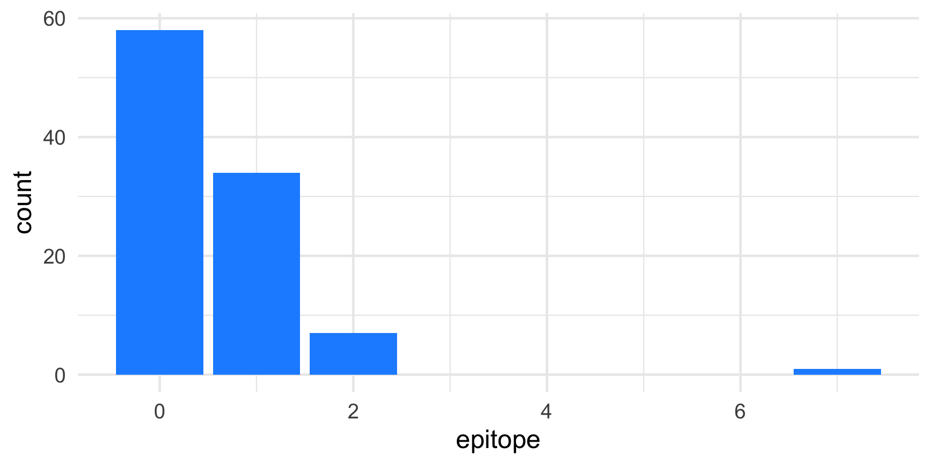
0 1 2 7
58 34 7 1 Statistical Modeling
Advanced Statistics and Data Analysis
Davide Risso
What is statistics
What is statistics
Statistics is the art of making numerical conjectures about puzzling questions.
Freedman et al., 1978.
The objective of statistics is to make inferences (predictions, decisions) about a population based on information contained in a sample.
Mendenhall, 1987.
What are statistical models
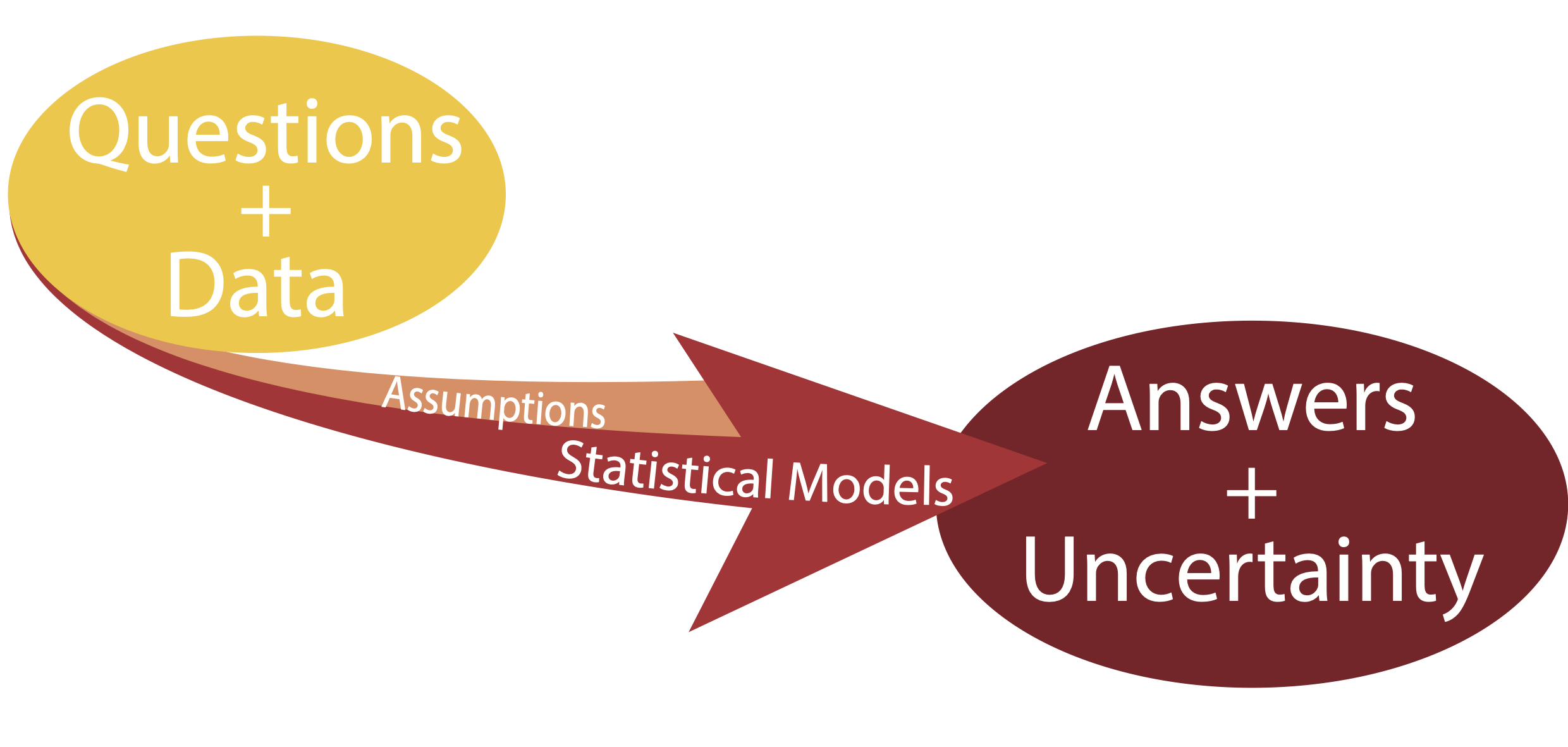
Statistical models are sets of equations involving random variables
Statistical models involve distributional assumptions
Given a question and a body of data statistical models can be used to provide answers along with measures of uncertainty.
What are statistical models
Statistical Models
Three key concepts: question, model, uncertainty
Far better an approximate answer to the right question, which is often vague, than an exact answer to the wrong question, which can always be made precise.
John W. Tukey, 1962.
All models are wrong, but some are useful.
George E. P. Box, 1987.
Statistical Inference
Statistical Inference
Statistical inference is the process of learning some properties of the population starting from a sample drawn from this population.
For instance, we may be interested in learning about the survival outcome of cancer patients, but we cannot measure the whole population.
We can however measure the survival of a random sample of the population and then infer or generalize the results to the entire population.
Statistical Inference
There are some terms that we need to define.
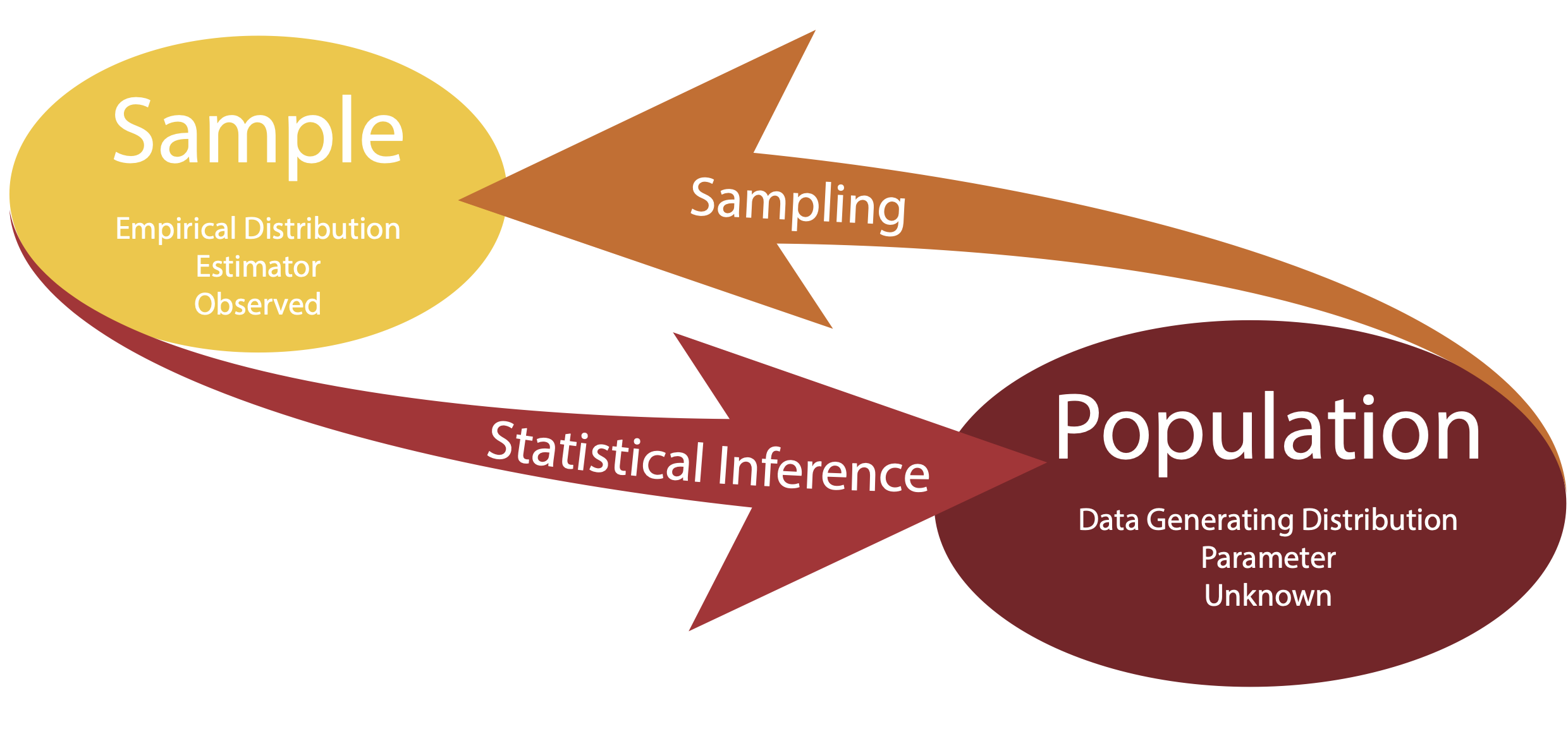
- The data generating distribution is the unknown probability distribution that generates the data.
- The empirical distribution is the observable distribution of the data in the sample.
We are usually interested in a function of the data generating distribution. This is often referred to as parameter (or the parameter of interest).
We use the sample to estimate the parameter of interest, using a function of the empirical distribution, referred to as estimator.
Statistical Inference
Statistical Inference
Statistical Inference
Parameter: unknown object of interest.
Estimator: data-driven guess at the value of the parameter.
In terms of mathematical notation, we often use Greek letters to refer to parameters and we use the same letter with the “hat” notation to refer to their estimate.
For instance, we denote with \(\hat{\theta}\) the estimator of the parameter \(\theta\).
Sometimes, you will find the notation \(\hat{\theta}_n\), when we want to emphasize that we are using a sample of \(n\) observations to estimate the parameter.
Example: Blood pressure in healthy individuals
Let’s assume that we want to estimate the average blood pressure of healthy individuals in the United States.
Let’s assume that we have access to blood pressure measurements for a random sample of the population (more on this later!).
- What is the parameter of interest?
- How can we estimate the parameter using the data in our sample?
Data generating distribution
The data generating distribution is unknown.
In nonparametric statistics we aim at estimating this distribution from the empirical distribution of the sample, without making any assumptions on the shape of the distribution.
However, it is often easier to make some assumptions about the data generating distribution. These assumptions are sometimes based on domain knowledge or on mathematical convenience.
One commonly used strategy is to assume a family of distributions for the data generating distribution, for instance the Gaussian distribution.
Random Variables
A variable is a measurement that describe a characteristic of a set of observations.
A random variable (r.v.) is a variable that measures an intrinsically random process, e.g. a coin toss.
Before observing the outcome, we will not know with certainty whether the toss will yield “heads” or “tails”, but that does not mean that we do not know anything about the process: we know that on average it will be heads half of the times and tails the other half.
If we refer to \(X\) as the process of measuring the outcome of a coin toss, we say that \(X\) is a random variable.
Statistical inference
It is somewhat confusing to talk about random variables in the context of statistical inference.
For instance, let’s say that we want to describe the height of a certain population. The height of an individual is not a random quantity! We can measure with a certain amount of precision the height of any individual.
What is random is the process of sampling a set of individuals from the population.
In other words, the randomness comes from the sampling mechanism, not from the quantity that we are measuring: if we repeat the experiment, we will select a different sample and we will obtain a different set of measurements.
Statistical modeling
The art of statistical modeling
Start with the data: exploratory data analysis (EDA).
Make probabilistic assumptions: choose a distribution.
Make inference: estimate the parameters of the distribution.
A simple example
When testing certain pharmaceutical compounds, it is important to detect proteins that provoke an allergic reaction.
The molecular sites that are responsible for such reactions are called epitopes.
ELISA assays are used to detect specific epitopes at different positions along a protein.
The protein is tested at 100 different positions, supposed to be independent.
We collect data from 50 patients, the reactions are summed at each location.
Start with the data: EDA
Make probabilistic assumptions
The Poisson distribution is a good model for counting rare events.
Would its distribution look similar to the one we observe?
First, we need to recall that the Poisson distribution depends on one parameter, namely \(\lambda\), which is also the mean (or expected value) of the distribution.
We can visually compare the observed distribution with a Poisson, with different values of \(\lambda\).
Check the goodness of fit
Observed data:
Check the goodness of fit
It seems that the simulated data have higher counts than our observed data.
We could try \(\lambda = 2\):
We could continue with all possible values of \(\lambda\) and choose the one that minimizes the differences between the observed and simulated data.
Compute the likelihood function
In other words, we want to compute the likelihood that the data come from the Poisson distribution with a given value of \(\lambda\), for any given value.
Since \(\lambda \in \mathbb{R}_+\), it is infeasible to try all possible values, and we can use a more elegant approach that uses the known form of the Poisson distribution to compute it.
Compute the likelihood function
What we want to compute is the probability that a Poisson r.v. with parameter \(\lambda\) will take the observed values. In R:
The function that we just computed is called the likelihood function and can be written as \[ L(\lambda, x) = \prod_{i=1}^n p(x_i), \] where \(p(x_i)\) is the probability mass function of a Poisson r.v.
Compute the log-likelihood function
For computational reasons, it is convenient to work with the log-likelihood, which sums the log of the pdf, and is usually indicated with the lowercase \(\ell\).
\[ \ell(\lambda, x) = \sum_{i=1}^n \log p(x_i). \]
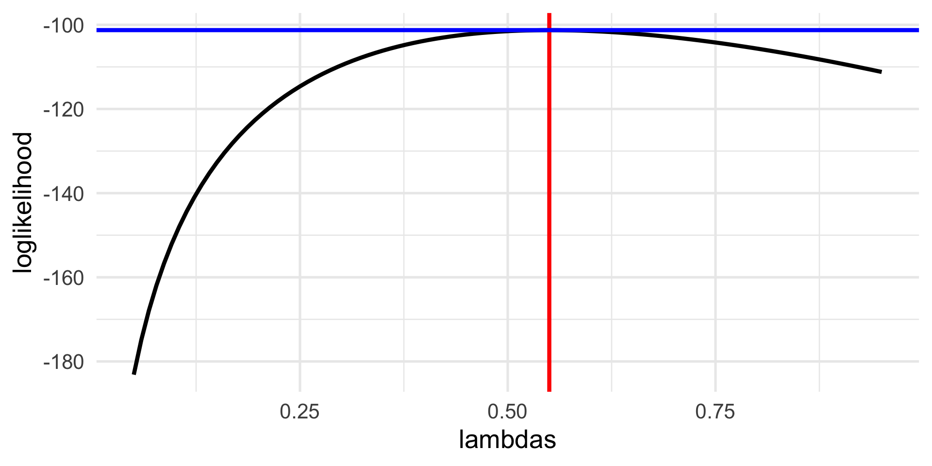
Search for the best \(\lambda\)
# Define a grid of lambdas
lambdas = seq(0.05, 0.95, length = 100)

# Compute the log-likelihood
loglikelihood = vapply(lambdas, loglik, numeric(1))

# Find the value that maximizes the log-likelihood
lambda_hat <- lambdas[which.max(loglikelihood)]
df <- data.frame(lambdas, loglikelihood)
p1 <- ggplot(df, aes(lambdas, loglikelihood)) +
    geom_line() +
    geom_vline(xintercept = lambda_hat, col = "red") +
    geom_hline(yintercept = max(loglikelihood), col="blue")
lambda_hat
[1] 0.55Search for the best \(\lambda\)
Classical statistics
What we have just done is to find a value of the parameter that maximizes the log-likelihood function.
Maths tells us that to find the maximum (or minimum) of a function we can compute its derivative.
In this case, the log-likelihood function is easy to compute from the Poisson pdf: \[ p(x) = \frac{1}{x!}\lambda^x e^{-\lambda}. \]
Hence \[ \ell(\lambda, x) = \sum_{i=1}^n -\lambda + x_i \log \lambda - \log(x_i!) \]
Classical statistics
We obtain \[ \ell(\lambda, x) = -n \lambda + \log \lambda \sum_{i=1}^n x_i - c, \]
from which we can derive \[ \frac{d \ell}{d\lambda} = -n + \frac{1}{\lambda} \sum_{i=1}^n x_i, \]
that leads to \[ \hat{\lambda} = \frac{1}{n} \sum_{i=1}^n x_i. \]
Hence, the sample mean.
Maximum Likelihood Estimation
We have just seen one of the most important procedures of statistical inference: Maximum Likelihood Estimation.
We call \(\hat{\lambda}\) the maximum likelihood estimate (MLE).
In the case of the Poisson distribution, the MLE is the mean of the sample.
Maximum Likelihood Estimation is a staple of modern statistics. We will see that in more complex models, we do not have a closed form solution for it and we will need to rely on numerical algorithms.
Another example
Suppose that we take a sample of \(n = 120\) males and test them for color blindness.
We can code with \(x_i=0\) if subject \(i\) is not colorblind, and with \(x_i = 1\) if subject \(i\) is colorblind.
Suppose that we obtain the data summarized in the following table.
cb
  0   1
110  10
Another example
- Assume that the data arise from a binomial r.v. with \(n=120\) trials and unknown success probability \(p\).
- What is your best guess at the value of \(p\)? Why?
- Use the
dbinomfunction in R to compute the likelihood for a grid of values of \(p\) and determine numerically the MLE. - Plot the log-likelihood function.
- Recall that the binomial pdf is \[ p(x) = \binom{n}{x} p^x (1-p)^{(n-x)} \]
- Use the derivative of the log-likelihood to compute the MLE.
To sum up
A statistical model uses probability distributions and random variables to provide a generative mechanism for the data that we observe.
Random variables are used to account for the statistical randomness that we have in our observed samples.
It is important to think carefully about what assumptions we are relying on when specifying a statistical model.
To sum up
The Maximum Likelihood Estimate (MLE) is the value of the parameter that maximizes the likelihood that the data arise from that distribution.
We obtain the MLE by maximizing the log-likelihood.
In simple models, we can use the derivative of the log-likelihood to obtain a closed-form estimate of the parameter.
In more complex models, we need to rely on numerical methods to maximize the log-likelihood.